Kuriko Iwai · 
Kuriko Iwai — Machine Learning Engineer · Founder of Kernel Labs
Production ML for engineers: fine-tuning, causal inference, and agents
From traditional ML to LLM fine-tuning, causal inference, and agentic systems—with ordered series, courses, and interactive labs.

Recommended Reads
What's New
Demystifying Apache Spark - Core Mechanics & RDD Execution Guide
Distributed Systems & Big Data Engineering — Deconstructing Spark Core Mechanics, Memory Management, and DAG Execution Lifecycle
Processing terabyte-to-petabyte-scale datasets on single-node architectures inevitably leads to severe disk I/O bottlenecks and memory exhaustion.
Apache Spark bypasses legacy MapReduce constraints by introducing an in-memory distributed computing engine powered by fault-tolerant Resilient Distributed Datasets (RDDs) and optimized DAG execution plans.
This comprehensive deep dive explores Spark's core runtime architecture, memory model, execution stages, Catalyst Optimizer mechanics, and production deployment modes.
Apache Spark is an open-source distributed computing system designed to quickly process large volumes of data which is hard to operate on a single machine.
Below diagram shows how Spark handles large-scale data conceptually:
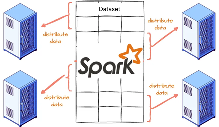
Figure A. Conceptual diagram of Apache Spark distributing large data chunks across physical machines (An original image edited by Kuriko IWAI)
Developed at UC Berkeley’s AMPLab in 2009 and later donated to the Apache Software Foundation, Spark distributes data and computations across multiple physical machines, allowing for parallel processing.
◼ Apache Spark Ecosystem
Apache Spark ecosystem has 3 main layers:
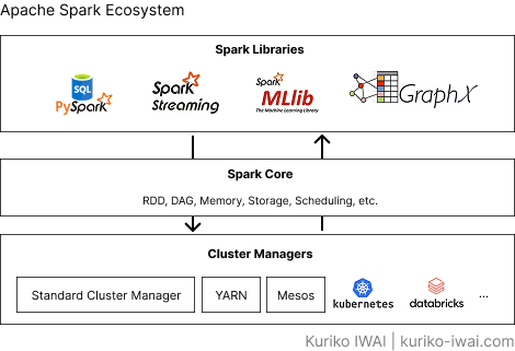
Figure B. The three-layer architecture of the Apache Spark Unified Ecosystem (Libraries, Core, Cluster Manager) (Created by Kuriko IWAI)
Spark Libraries (also known as the Spark Unified Libraries) (top, Figure B) consist of 4 high-level components built on top of a common engine:
Spark SQL & DataFrames: Structured query processing, schema management, and relational data operations powered by the Catalyst Optimizer and Tungsten execution engine.
Spark Streaming / Structured Streaming: Real-time stream processing that unifies batch and micro-batch/continuous processing with end-to-end exactly-once semantics.
MLlib (Machine Learning Library): Scalable machine learning algorithms, feature engineering tools, and standardized Pipeline abstractions for model training and evaluation.
GraphX: A distributed graph processing engine and API for graph-parallel computation and network analysis.
These high-level libraries call Spark Core (middle, Figure B) to translate code into data transformation and execute plans.
Then Spark Core requests and manages resources through the Cluster Manager (bottom, Figure B), schedule and execute tasks across worker nodes.
I'll walk you through this mechanism and process in the next section.
How Spark Core Works - The Spark Application Architecture
Spark operates using a master-worker architecture controlled by a driver program and executed across multiple worker nodes.
The below diagram shows the high level runtime architecture of Apache Spark:
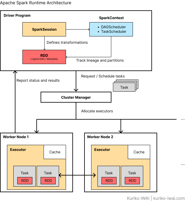
Figure C. High-level runtime architecture of Apache Spark showing driver, cluster manager, and executors (Created by Kuriko IWAI)
As Figure C shows, there are 5 primary components:
Driver program (master node) (top, Figure C),
Cluster manager (master node/orchestrator) (middle, Figure C),
Worker node (bottom, Figure C),
Executor, and
Task.
◼ Driver Program
Driver program (or called driver) is the central coordinator node of a Spark application.
It translates code into DAG, tasks, and coordinates execution;
Instantiates the SparkSession with its underlying SparkContext.
Analyzes data transformations and actions.
Breaks the execution into stages and tasks (each of which will be handled by an executor).
Schedules tasks and sends them to individual executors.
Collects final results.
◼ Cluster Manager
Cluster manager is the external service responsible for acquiring and allocating CPU/RAM resources across the worker nodes in the cluster.
It oversees the cluster of machines running the Spark application.
Spark can work with various cluster managers:
Standalone: Spark's built-in, simple cluster manager.
YARN: Hadoop's resource manager (common in traditional enterprise setups).
Kubernetes (k8s): Container-based resource orchestration.
Databricks Managed Cluster Manager: Auto-scaling cluster management native to Databricks.
◼ Worker Nodes
Worker nodes are the physical or virtual machines in the cluster that host executor processes.
They provide CPU, memory, and storage resources to run workloads.
They do not execute business logic directly; instead, they launch and manage executor processes.
◼ Executors
An executor is a dedicated distributed Java Virtual Machine (JVM) process launched on a worker node for a specific Spark application.
As Figure C shows, executors execute tasks the driver assigns and report their status and results:
Runs individual Tasks assigned by the Driver across multiple CPU threads.
Stores cached DataFrames/RDD partitions in memory (RAM) or disk.
Persists until the application finishes or is dynamically terminated.
Each Spark application has its own set of executors, and a single worker node can host multiple executors.
◼ Tasks
A task is the smallest individual unit of work in Spark.
A single task represents the execution of a set of transformations on a single partition of data.
Figure C shows at least 4 tasks are created in 4 separate partitions, as a Resilient Distributed Dataset (RDD) has 4 partitions.
When an RDD (or DataFrame) has 100 partitions, Spark creates 100 tasks to process that stage.
The next section explains how RDD works.
Resilient Distributed Dataset (RDD)
Resilient Distributed Dataset (RDD) is the fundamental, low-level data abstraction in Apache Spark.
The below diagram shows how RDDs handle its core operations:
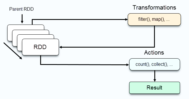
Figure D-1. RDD abstraction and core operations (Lazy transformations vs eager actions)
RDD is an immutable, read-only collection of data partitioned and distributed across worker nodes of a cluster.
RDD holds any type of data like Scala, Java, or Python objects (e.g., integers, strings, custom classes, or key-value tuples) in memory for as long and as much as possible.
◼ Core Operations - Transformations and Actions
As Figure D-1 shows, operations on an RDD fall into 2 categories:
Transformations (lazy), and
Actions (eager).
Transformations (and Lazy Evaluation)
Transformations are operations that create a new RDD from an existing one.
Examples include:
.map()
.filter()
.groupByKey()
.select()
.filter()
.join()
Transformations are lazily evaluated; Spark records the operation in a DAG, but does not execute it immediately.
Actions
Actions are operations that compute a result and return it to the Driver Program or write it to storage.
Examples include:
.collect()
.count()
.saveAsTextFile().
Calling an action triggers actual computation across the cluster.
▫ Operational Flow
When we define the RDD, its inside data is not transformed immediately until an action triggers the execution.
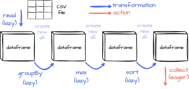
Figure D-2. Operational execution flow of RDD transformations, DAG building, and lineage graph evaluation
Figure D-2 shows that transformations first build a DAG plan, and when an action is called, the data is finally processed.
This approach allows Spark to determine the most efficient way to execute the transformations.
◼ Fault Tolerance
RDDs achieve fault tolerance through lineage.
As Figure D-2 shows, Spark forms the dependency lineage graph by keeping track of each RDD’s dependencies on other RDDs, which is the series of transformations that created the RDD.
When a worker node crashes and data in memory is lost, Spark simply uses this graph to recompute only the crashed node, completely skipping restarting the entire application.
◼ Benefits of Immutability
We know that RDDs are immutable; once created, it cannot be modified.
This means that any operation on an RDD produces a brand-new RDD rather than altering the existing one ("create new df" in Figure D-2).
This helps Spark in 3 ways:
Concurrent processing: Immutability keeps data consistent across multiple nodes and threads, avoiding complex synchronization and race conditions. Spark can call multiple CPU cores to compute data simultaneously.
Fault tolerance: Each transformation creates a new RDD, preserving the lineage and allowing Spark to recompute lost data reliably.
Functional programming: RDDs follow functional programming principles that emphasize immutability, making it easier to handle failures and maintain data integrity.
◼ Anatomy of an RDD - The 5 Internal Properties
Every RDD in Spark is defined by 5 core properties:
List of partitions: Defines parallelism (How many tasks will run).
Computation function: Defines logic (How to iterate over and transform data).
Dependencies: Defines lineage & fault tolerance (How to reconstruct lost partitions).
Partitioner (optional): Defines data distribution (For key-value RDDs, how key-value keys are grouped across nodes).
Preferred locations (optional): Defines task placement (Where to run tasks to minimize network I/O).
◼ Partitions
Partitions is the array of discrete subsets into which the dataset is logically divided.
Spark cannot process a multi-terabyte file as a single monolith, so it splits the data into atomic units called partitions.
When an RDD is created, Spark divides the data into multiple chunks, known as partitions. Each partition is a logical data subset and can be processed independently with different executors. This enables Spark to perform operations on large datasets in parallel.
When a stage runs, Spark assigns one task per partition.
If an RDD has 100 partitions, Spark will launch 100 tasks to process them, running as many concurrently as there are available CPU cores/executor slots.
1from pyspark.sql import SparkSession
2
3# define spark session and context
4spark = SparkSession.builder.appName("app").getOrCreate()
5sc = spark.sparkContext
6
7# create an rdd with 4 explicit partitions
8rdd = sc.parallelize(range(1, 1000), numSlices=4)
9
For example, reading a 1 GB file with a 128 MB block size produces an RDD with 8 partitions.
◼ Computation Function
Computation function is an internal function that defines how to calculate the data for a given partition from its parent data.
Because RDDs are evaluated lazily, Spark doesn't immediately hold all data in memory; instead, it holds the recipe for computing it.
In the below code snippet, when the compute function is built, no worker node runs computation. Only when .collect() is called, the computation is triggered:
1from pyspark.sql import SparkSession
2
3# define spark session and context, create an rdd
4spark = SparkSession.builder.appName("app").getOrCreate()
5sc = spark.sparkContext
6rdd = sc.parallelize(range(1, 1000), numSlices=4)
7
8# build the compute function (even numbers x 10)
9filtered_rdd = rdd.filter(lambda x: x % 2 == 0)
10mapped_rdd = filtered_rdd.map(lambda x: x * 10)
11
12# calling .collect triggers the compute() method on each partition
13result = mapped_rdd.collect()
14
◼ Dependencies (Lineage)
Dependencies (or lineage) is a list of parent RDDs that the current RDD depends on, along with the nature of that dependency.
RDDs track their history to provide fault tolerance and build the DAG.
Spark classifies dependencies into two types:
Narrow dependency (or called narrow transformation): Each partition of the parent RDD is used by at most one partition of the child RDD (e.g., map(), filter()). Data stays local on the node; no network shuffle is needed.
Wide dependency (or called wide transformation): Multiple child partitions depend on data from a single parent partition (e.g., groupByKey(), join()). This triggers a shuffle, moving data across the network.
1from pyspark.sql import SparkSession
2
3# define spark session and context
4spark = SparkSession.builder.appName("app").getOrCreate()
5sc = spark.sparkContext
6
7# parent rdd
8rdd1 = sc.parallelize([("USA", 1), ("Canada", 2), ("USA", 3)])
9
10# narrow dependency: map() doesn't move data across network nodes
11rdd2 = rdd1.map(lambda x: (x[0], x[1] * 100))
12
13# wide Dependency: reduceByKey() requires a shuffle across the network
14rdd3 = rdd2.reduceByKey(lambda a, b: a + b)
15
16
17# inspect dependencies
18dependencies = rdd3._jrdd.dependencies()
19dependency_type = dependencies[0].getClass().getSimpleName()
20# dependncy_type returns ShuffleDependency
21
◼ Partitioner
Partitioner is an object that controls how key-value pair elements (RDD[(K, V)]) are routed to specific partition IDs.
For plain RDDs (e.g., text lines), the partitioner is None.
For key-value RDDs subjected to shuffle operations (like .reduceByKey() or .join()), Spark uses a partitioner:
HashPartitioner: Calculates hash(key) % numPartitions to send rows with identical keys to the exact same partition/node.
RangePartitioner: Sorts keys into ordered range buckets across partitions (used in .sortByKey()).
When two datasets are joined and already share the same partitioner, Spark skips the costly network shuffle during the join.
1from pyspark.sql import SparkSession
2
3# define spark session and context
4spark = SparkSession.builder.appName("app").getOrCreate()
5sc = spark.sparkContext
6
7# mock data
8data = [("A", "Emp1"), ("B", "Emp2"), ("A", "Emp3")]
9
10# plane rdd
11raw_rdd = sc.parallelize(data)
12raw_rdd.partitioner
13# -> returns None
14
15
16# custom partition function to map key to rdd
17def custom_partition_func(key: str) -> int:
18    return 0 if key == "A" else 1
19
20# apply an explicit partitioner
21partitioned_rdd = raw_rdd.partitionBy(
22    numPartitions=2,
23    partitionFunc=custom_partition_func,
24)
25partitioned_rdd.partitioner
26# -> returns ``
27# confirming a partitioner object is actively attached to the rdd.
28
◼ Preferred Locations
Preferred locations are metadata specifying the physical IP addresses/hostnames where a given partition's source data resides.
Spark enforces the principle of data locality, indicating that moving computation to the data is cheaper than moving data to the computation.
When reading from storage systems like HDFS or Delta/S3, Hadoop Distributed File System (HDFS) tells Spark:
Block 1 of File A is physically stored on Node-101.
Spark’s scheduler reads preferredLocations() for Partition 1, sees Node-101, and attempts to assign Task 1 to an executor running on Node-101.
Locality levels: Spark attempts assignments in order of priority:
PROCESS_LOCAL (Data is already cached in the executor JVM).
NODE_LOCAL (Data is on the same physical server disk/HDFS block).
RACK_LOCAL (Data is on the same rack).
ANY (Data must be transferred over the network from another node).
1from pyspark.sql import SparkSession
2
3# define spark session and context
4spark = SparkSession.builder.appName("app").getOrCreate()
5sc = spark.sparkContext
6
7# read data from a distributed/locality-aware file system (e.g., HDFS/S3)
8file_rdd = sc.textFile("hdfs://namenode:9000/data/mock.csv")
9
10# get the jave rdd instance
11java_rdd = file_rdd._jrdd
12
13# query preferred locations for Partition 0
14first_partition = java_rdd.partitions()[0]
15preferred_hosts = java_rdd.preferredLocations(first_partition)
16
17# preferred_hosts: ['datanode101.internal', ...]
18
Shipping AI Systems?
I help teams design and deploy scalable ML / RAG / LLM pipelines and MLOps infrastructure.
Or explore:
- Dive deeper 👉 Research Archive
- Learn by building 👉 AI Engineering Masterclass
- Try it live 👉 Playground
The Execution Lifecycle: From Code to Tasks
This section explains a complete, step-by-step breakdown of the Spark Execution Lifecycle, tracing the exact sequence of events from when we submit code to when results are returned.
◼ Step 1. Initializing the Driver
First, we submit a Spark application (via spark-submit, a Databricks Notebook cell, or an IDE).
The driver program process starts up, either locally or on a designated cluster node based on your deployment mode (I'll later explain).
Then, the driver creates a SparkSession and underlying SparkContext, which contacts the Cluster Manager to request compute resources.
1from pyspark.sql import SparkSession
2
3# driver process initializes to create a SparkSession
4spark = SparkSession.builder \
5    .appName("app") \
6    .master("local[*]") \
7    .config("spark.executor.memory", "2g") \
8    .getOrCreate()
9
10# create a SparkContext
11sc = spark.sparkContext
12
13# the driver immediately transitions to step 2. executor allocation by requesting cpu cores and ram from the cluster manager.
14
◼ Step 2. Executor Provisioning & Registration
The cluster manager launches executor processes inside separate JVMs across the designated worker nodes.
Each executor registers back with the driver’s TaskScheduler, reporting its available CPU core slots and RAM capacity.
The cluster is now active, and the Driver is ready to parse your application code.
◼ Step 3. Building DAG
Spark reads each transformation then builds a node in a DAG, which tracks the lineage graph.
1# mock data
2mock_data = [("US", 10), ("CA", 20), ("US", 30), ("UK", 15)]
3
4# create a base rdd
5base_rdd = sc.parallelize(mock_data, numSlices=2)
6
7# create lineage graph
8filtered_rdd = base_rdd.filter(lambda x: x[1] > 12)
9mapped_rdd = filtered_rdd.map(lambda x: (x[0], x[1] * 2))
10
◼ Step 4. Catalyst Optimization
For DataFrame and SQL operations, the catalyst optimizer builds and optimizes the physical execution plan.
1# define a DataFrame pipeline
2df = spark.createDataFrame([
3    ("Alice", "Engineering", 90000),
4    ("Bob", "Engineering", 120000),
5    ("Charlie", "Sales", 80000)
6], ["name", "department", "salary"])
7
8# transformations build the catalyst logical plan
9processed_df = df \
10    .filter(df.salary > 85000) \
11    .select("name", "department")
12
13# inspect the complete catalyst planning pipeline
14processed_df.explain(extended=True)
15# output shows:
16# 1. Parsed Logical Plan
17# 2. Analyzed Logical Plan
18# 3. Optimized Logical Plan (Filter pushdown / column pruning)
19# 4. Physical Plan (WholeStageCodegen execution strategy)
20
◼ Step 5. Creating Stages
An action is called to trigger the DAGScheduler on the driver.
The DAGScheduler evaluates the logical DAG and breaks it into physical stages.
Then, the DAGScheduler passes each stage to the TaskScheduler.
◼ Step 6. Creating Tasks
The TaskScheduler splits each stage into individual tasks.
Each Task corresponds 1:1 with a single data partition.
The TaskScheduler then evaluates data locality via preferredLocations to figure out which executor holds or is closest to the physical data partition.
The driver dispatches these tasks to the available executor slots across the network.
1# wide transformation (reduceByKey) creates a shuffle boundary
2grouped_rdd = mapped_rdd.reduceByKey(lambda a, b: a + b)
3
4# calling an action (.collect()) triggers DAGScheduler & TaskScheduler execution
5result = grouped_rdd.collect()
6
◼ Step 7. Executing Tasks in Parallel
Executors receive the serialized task code from the driver, and run the tasks in parallel across their available CPU threads.
If a task requires caching (via .cache()), the partition results are saved in the executor’s memory storage space.
◼ Step 8. Shuffle for Multi-stage Execution
If the job has multiple stages, executors exchange data over the network during the shuffle phase.
Stage 1 tasks finish writing their output partitions into shuffle files on local executor disks.
Then, Stage 2 tasks wake up and pull their corresponding key-partitioned data over the network from Stage 1 executors.
Stage 2 tasks execute their logic once all required shuffle data is fetched.
1# inspect how data partitions were evaluated during execution across tasks
2def inspect_executor_task(partition_index, iterator):
3    data = list(iterator)
4    yield f"task on partition {partition_index} processed {len(data)} items: {data}"
5
6# collect partition execution layout from executors
7task_logs = grouped_rdd \
8    .mapPartitionsWithIndex(inspect_executor_task) \
9    .collect()
10
◼ Step 9. Results
Final output tasks complete and send their results back.
If saving to storage, executors directly write output files to the target file system/Data Lake in parallel.
If returning to the driver, executors serialize their output partition results back to the driver memory space.
1# write final DataFrame to persistent storage (distributed write across executors)
2df.write.mode("overwrite").parquet("/tmp/output_data.parquet")
3
◼ Step 10: Shutting Down the Application
The job reaches completion or the script finishes.
The SparkSession is closed via .stop() or notebook termination.
The driver notifies the cluster manager to release all allocated executor JVM processes and free CPU/RAM resources across the worker nodes.
1# stop SparkSession to shut down Executors and release driver resources
2spark.stop()
3
Spark Execution Mode
Spark offers different execution modes:
Cluster mode,
Client mode, and
Local mode
which can run the execution lifecycle in its own way.
Below diagram shows the high-level concept, where the execution mode control where the driver runs, then the driver runs Spark lifecycle:
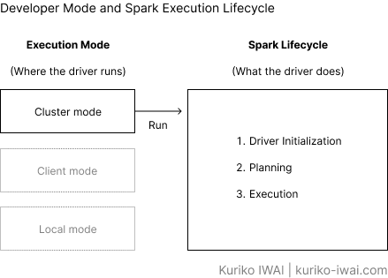
Figure E. Conceptual overview of Spark Application execution modes and its lifecycle (Created by Kuriko IWAI)
◼ Cluster Mode
Cluster mode is the production standard mode where the driver process is launched on a worker node within the cluster alongside the executor processes:
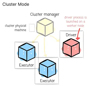
Figure F-1. Spark cluster mode execution architecture (Driver running inside the worker node)
In cluster mode, the client submits the job and disconnects; then the cluster manager handles all the processes related to the Spark application:
▫ Best Used For:
Automated production pipelines and scheduled batch jobs (e.g., airflow jobs) where network latency between driver and executors must be minimized.
◼ Client Mode
Client mode is the mode where the driver remains on the client machine that submitted the application:
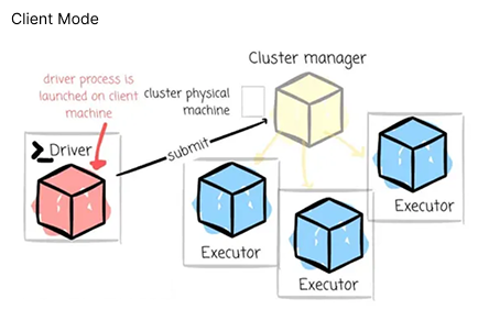
Figure F-2. Spark client mode execution architecture (Driver running on submitter edge machine).
In client mode, the driver process runs on the submitter's machine (e.g., laptop, an edge node, or a Databricks Notebook driver node), outside the worker cluster pool.
This setup requires the client machine to maintain the driver process throughout the application’s execution.
▫ Best Used For:
Interactive querying, data exploration, and REPL/Notebook development (e.g., Databricks interactive notebooks, Jupyter) where instant feedback is required.
◼ Local Mode
Local mode is the mode where the entire Spark application is ran on a single machine, achieving parallelism through multiple threads.
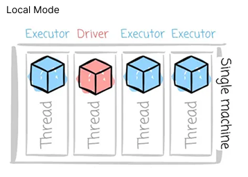
Figure F-3. Spark local mode architecture (Driver and executors co-existing in a single JVM process)
In local mode, there is no real cluster or cluster manager.
The driver and executor run inside the exact same JVM process on a single machine.
▫ Best Used For:
Unit testing, debugging PySpark code locally, and small-scale development on your laptop without spinning up a cluster.
◼ Comparing Execution Modes
Below table compares each execution mode with use case:
Feature | Cluster Mode | Client Mode | Local Mode |
Where Driver Runs | Inside a Worker Node in the cluster | On the edge/gateway machine (laptop/notebook) | Inside a single local JVM thread pool |
Where Executors Run | On Worker Nodes across the cluster | On Worker Nodes across the cluster | Same JVM process as the Driver |
Driver-Executor Latency | Extremely Low (Same cluster network) | Higher (Crosses edge-to-cluster network) | Zero (In-memory thread switching) |
Primary Use Case | Production batch & streaming jobs | Interactive notebooks & debugging | Local unit testing & development |
Table 1. Architectural comparison of Apache Spark execution modes (Cluster vs. Client vs. Local) (Created by Kuriko IWAI)
Shipping AI Systems?
I help teams design and deploy scalable ML / RAG / LLM pipelines and MLOps infrastructure.
Or explore:
- Dive deeper 👉 Research Archive
- Learn by building 👉 AI Engineering Masterclass
- Try it live 👉 Playground
Wrapping Up
Spark was built to address the severe latency and disk I/O bottlenecks of classical MapReduce architectures.
Rather than writing intermediate state back to persistent disk after every map and reduce phase, Spark performs in-memory computing using persistent fault-tolerant abstractions.
Its typical use cases involve:
Large-scale ML feature engineering: Computing complex aggregations, window functions, and embeddings over billions of rows.
Distributed ML model inference: Scoring massive batch datasets using distributed PySpark UDFs or Spark Predictor pipelines.
Real-time feature stores: Streaming continuous features into online/offline storage using Structured Streaming.
ETL & Data lakehouse ingestion: Cleaning, deduplicating, and converting raw JSON/CSV logs into optimized Delta Lake format.
◼ Common Pitfalls
Although Spark is beneficial to handle large datasets, there are some common pitfalls.
▫ High Memory Footprint
JVM garbage collection overhead, memory leaks in Python worker processes, or unoptimized caching can cause Driver/Executor OutOfMemory (OOM) failures.
▫ Handling Skewed Data
If a key distribution is uneven (e.g., null keys or dominant IDs), one executor processes 90% of the data while others sit idle, causing severe stragglers.
▫ Small File Problem
Generating thousands of small partition files degrades read throughput and metastore query planning.
▫ PySpark Serialization Overhead
Converting data between JVM execution layers and Python worker processes (Py4J / IPC) introduces performance overhead when using non-vectorized Python UDFs.
◼ When to Use Spark
Understanding when to use Spark—and when not to—is important given pros and cons of Spark.
▫ Use Spark When:
Data size exceeds single-node capacity: Your data cannot fit into high-memory VMs (e.g., 256GB+ RAM).
Workloads require distributed compute: Feature calculations require distributed joins across massive multi-table data models.
SLA-critical streaming is required: Real-time processing with low-latency streaming pipelines.
▫ Avoid Spark When:
Data fits easily in single-node RAM: Datasets under ~20–50 GB can be processed faster with single-node tools like Pandas, Polars, or DuckDB without cluster initialization and serialization overhead.
Purely iterative single-node ML algorithms: Training standard, non-distributed Scikit-Learn models on small datasets.
How to Solve Time-Varying Confounding & Mediator Bias in Longitudinal ML Pipelines
[Series] Causal Machine Learning - 3. De-Biasing Sequential Telemetry and Multi-Period Decisions
Standard machine learning and static causal models fail in multi-period sequential systems where time-varying telemetry acts simultaneously as a mediator and a confounder.
Naive feature flattening or standard conditioning triggers mediator-blocking bias and collider stratification bias—severely distorting downstream policy evaluation.
This guide explores the mathematics of sequential exchangeability, time-varying inverse propensity weighting (IPTW), and Marginal Structural Models (MSMs) with a production-ready Python implementation.
Time-varying trap (or time-varying confounding) indicates a complex scenario in sequential, multi-period data where a variable measured over time acts simultaneously as a mediator and a confounder.
Below diagram shows how system states evolve over a multi-period horizon:
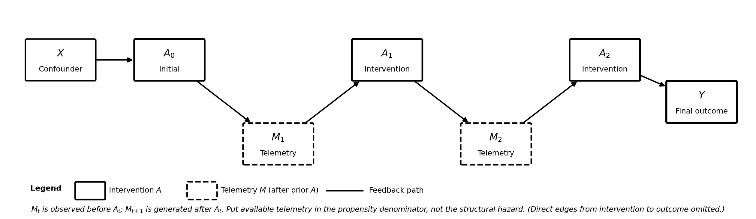
Figure A. Longitudinal Directed Acyclic Graph (DAG) showing time-varying confounding and telemetry dual-roles in enterprise employee retention (Created by Kuriko IWAI)
Let us consider an enterprise employee retention pipeline across two time steps.
The figure include key components:
Confounder X: The employee's background and professional experience.
Initial intervention A_0: Day1 onboarding program assignment.
Month-1 telemetry M_1: Engagement of the employee (M_1 = 1 indicates high engagement).
Month-1 intervention A_1: Manager's check-ins in Month 1.
Final outcome Y: Retention of the employee at the end of temporal horizon (i.e., T = 12 months).
◼ The Dual-Role of Telemetry - Mediator AND Confounder
Here, M_1 is a mediator because the initial intervention improves it.
For instance, if an employee had good onboarding experience, they'd be likely to engage more (A_0 = 1 → M_1 = 1).
But M_1 is also a confounder because a sudden drop in engagement could trigger A_1 (manager's check-ins) and directly lower retention Y.
M_1 is directly impacted by the past interventions, but also impacts on future interventions, and hence, the final outcome.
Because M_1 plays both roles over time, static feature-flattening models fail to isolate the true causal effect of this continuous sequences.
Why Standard ML Models Break
In static ML, we only worry about baseline confounder X.
But in sequential systems we saw in the previous section, past interventions pollute future states.
This makes static ML face a structural dilemma.
◼ The True Causal Effect
Imagine we have 1,000 software engineers in our staffing pipeline.
When we split them into two groups:
Group 1. (500 engineers) Receives intensive onboarding (A_0 = 1), and
Group 2. (500 engineers) Receives standard onboarding (A_0 = 0).
Below diagram demonstrates how the true causal effect is measured for retention at temporal horizon T:
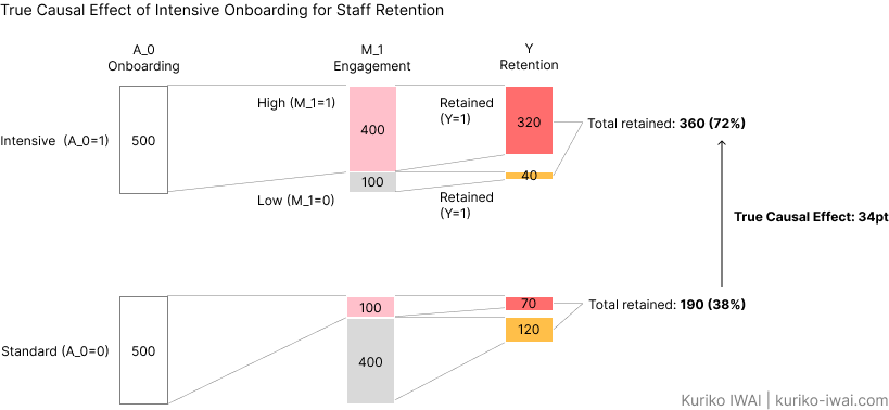
Figure B-1. True total causal effect of multi-period interventions on long-term retention (Created by Kuriko IWAI)
Among 500 engineers under the intensive onboarding (upper row, Figure B-1), 400 engineers had high engagement at Month 1, and 320 engineers were retained.
The remaining 100 developers had low engagement, but 40 engineers were retained.
So, in total, the intensive onboarding achieved 72% of retention rate; compared to 38% of standard onboarding (bottom row, Figure B-1), boosting the retention rate by 34 points.
◼ Mediator-blocking Bias
Native ML models control for M_1 by including M_1 in the feature set.
However, this accidentally blocks the indirect causal path of the initial intervention A_0:
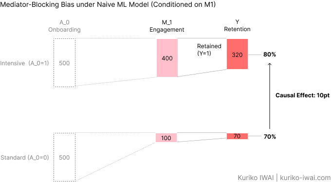
Figure B-2. Mediator-blocking bias misestimates causal effect due to covariate over-adjustment (Created by Kuriko IWAI).
Figure B-2 demonstrates mediator-blocking bias (or over-adjustment bias) where when an ML model conditioned on M_1, it completely misses the benefit of intensive onboarding (A_0 = 1) which drives 80% of developers into high engagement (M_1 = 1), instead of just 20%.
▫ Mathematical Background of Mediator-blocking Bias
Suppose our data science team attempts to evaluate the retention strategy by fitting a standard multi-variable regression model:
where β's represent weights assigned to each variable and k represents temporal horizon such as k=12.
Eq. 1 includes M_1 because we correctly identify that M_1 is a confounder for A_1.
This, however, blocks the indirect causal path from A_0 to Y, dampening weight β_0 which measures the Controlled Direct Effect (CDE) of A_0 on the final outcome.
On the other hand, the model attributes credit for M_1, even though A_0 actually caused M_1, assigning a large value to β_1.
Stakeholders looking at large β_1 might say: "Month 1 engagement (M_1) drives employee retention. Let's focus on engagement.", missing the fact that M_1 was a result of the onboarding program (A_0).
Metric | Ground Truth | Naive ML Model Conditioned on M_1 | Impact / Business Risk |
|---|---|---|---|
ROI for Intensive Onboarding (A_0 = 1) | +35pt boost | +10pt boost | Executive leadership cancels the onboarding program, incorrectly believing it provides negligible long-term value. |
Causal Path Measured | Total Causal Effect | Controlled Direct Effect | The primary mechanism (A_0 → M_1) is blocked and hidden by feature set inclusion. |
Handling of M_1 | Recognized as dynamic Mediator AND Confounder. | Treated as a static baseline covariate. | Feature flattening induces structural bias in continuous policy evaluation. |
Table 1. Ground Truth vs. Naive ML Conditioning on Time-Varying Mediators (Created by Kuriko IWAI)
◼ Selection Bias
When we exclude M_1 from the feature set, the estimation of the secondary intervention A_1 suffers from uncontrolled baseline confounding.
Selection bias occurs in two situations:
Confounder selection bias: Failing to control for baseline X when assigning onboarding, so the model analyzes non-randomly selected samples.
Collider stratification bias: Conditioning on a variable that creates a fake correlation between two independent variables; for example, evaluating manager interventions (A_1) by filtering the dataset strictly to low-engagement developers (M_1 = 0).
◼ Confounder Selection Bias
Suppose Senior Engineers (X = 1) inherently retain at higher rates (80%), but managers preferentially send Junior Engineers (X = 0) to the intensive onboarding program (A_0 = 1) because they need more help:
Senior Engineers (X = 1, 500 total): Naturally retained at 80%. Only 100 were assigned to the intensive program.
Junior Engineers (X = 0, 500 total): Naturally retained at 40%. 400 were assigned to the intensive program.
Below diagram demonstrates confounder selection bias:
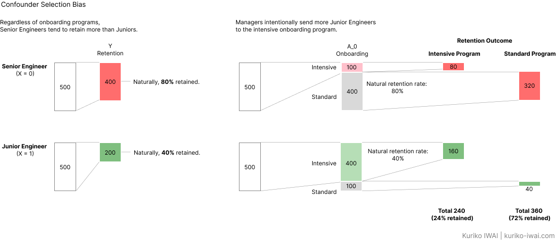
Figure C-1. Confounder selection bias resulting from non-random treatment assignment across baseline demographics (Created by Kuriko IWAI)
When the analyst simply compares retention rates after the intensive and standard onboarding program, standard has much higher rate (72%, right, Figure C-1) than intensive (24%, middle, Figure C-1).
But the truth is that the sample receiving the intensive program was heavily biased toward Junior Engineers who naturally leave at higher rates.
Here, intensive onboarding wasn't failing at all—it was handed a fundamentally harder population: Junior Engineers.
◼ Collider Stratification Bias
Collider stratification bias is a subtle form of selection bias where conditioning on a middle variable (M_1) artificially creates an inverted correlation between two unlinked factors.
Suppose two unlinked factors cause low engagement (M_1 = 0):
Standard onboarding (A_0 = 0), and
Personal burnout / external hardship (U = 1).
Suppose leadership asks:
Let's evaluate how manager check-ins affect retention for at-risk engineers with low engagement.
By restricting the analysis strictly to low-engaging engineers (M_1 = 0), the model confuses that the intensive onboarding causes low engagement.
But in reality, these engineers had low engagement not because of poor onboarding, but because of personal burnout (U = 1, left, Figure C-2).
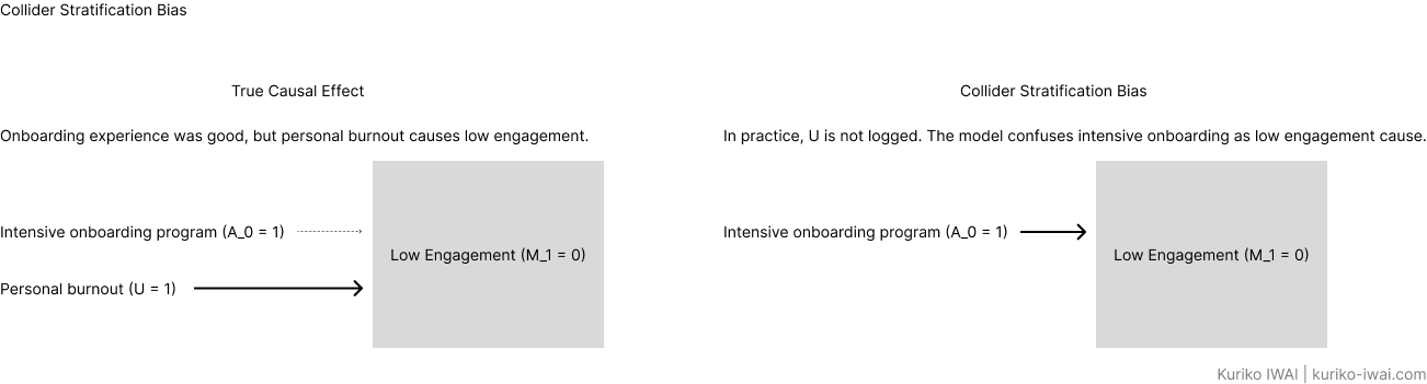
Figure C-2. Collider stratification bias induced by conditioning on intermediate telemetry affected by unobserved confounders (Created by Kuriko IWAI).
Here, M_1 is a collider because two separate factors (A_0 and U) point directly into it.
And U represents factors like personal family emergencies, mental fatigue, bad team dynamics, or sudden external hardships.
In real-world enterprise telemetry, U is rarely logged or quantifiable.
Because U remains unobserved and hence, omitted from the regression model, filtering on M_1 = 0 forces A_0 to act as a proxy of U.
So, how can we know if we have recorded enough history to calculate true cause-and-effect?
The Rules of Identification: Sequential Exchangeability
Sequential exchangeability tackles these challenges by structurally completing the causal pipeline, extending Judea Pearl's backdoor criterion across time t:
where \bar{H}_t represents historical trajectory up to time step t:
where \bar{A}_{t-1} and \bar{M}_t represent a complete sequence of past interventions up to step t-1 and post-treatment intermediate states up to step t, respectively.
In this concept, the decision to assign intervention A_t is independent of the potential counterfactual outcome Y(\bar{a}), indicating that there's no unobserved confounders affecting intervention A_t at any stage of the pipeline, once historical trajectory is defined.
◼ How Sequential Exchangeability Solves Both Biases
Sequential exchangeability is the theoretical backbone that powers Inverse Probability of Treatment Weighting (IPTW) and Marginal Structural Models (MSMs).
▫ Eliminating Selection Bias
First, it eliminates selection bias at every step.
IPTW calculates time-varying weights:
These weights construct a synthetic pseudo-population where intervention A_t is pseudo-randomized relative to past history.
This can strip away the selection bias because A_t is no longer determined by past history \bar{H}_t, breaking the confounding links that caused the bias in the first place.
▫ Eliminating Mediator-blocking bias
Instead of putting M_1 directly into the regression model, sequential exchangeability uses M_1 only to construct the propensity weights W_t.
For a two-stage longitudinal pipeline with initial intervention A_0, intermediate state M_1, and secondary treatment A_1, the cumulative unstabilized weight W is the product of the inverse propensity scores at each time step:
where:
Weight at time t=0 (W_0) for individual i inversely models the probability of receiving initial intervention A_0 given baseline confounder X, and
Weight at time t=1 (W_1) for individual i inversely models the probability of receiving secondary treatment A_1 given the full prior trajectory \bar{H}_1 = {X, A_0, M_1}.
This unstabilized weight can produce extreme values (large variance) if some intervention probabilities are very small.
In practice, we use Stabilized Weights (SW), which replace the numerator 1 in Eq. 3.2 with the probability of the current intervention conditioned only on past intervention history:
where A_0 and A_1 represent interventions at t = 0 and t = 1 respectively.
Eq 3.3.1 can be generalized with T time steps:
Once SW_i (Eq. 3.3.2) is calculated for every individual, we can fit a weighted regression model for final outcome Y using only the intervention history variables (A_0, A_1), completely excluding M_1:
Because M_1 was used to construct SW_i (included in the past history), the sample is reweighted to break the confounding links, while leaving the mediator path (A_0 -> M_1 -> Y) open.
Now, β_1 successfully captures the true total causal effect (+34pt) of the intensive onboarding program.
Also, the model does not stratify on post-treatment status, preventing A_0 from becoming a proxy for unobserved factors (U).
Shipping AI Systems?
I help teams design and deploy scalable ML / RAG / LLM pipelines and MLOps infrastructure.
Or explore:
- Dive deeper 👉 Research Archive
- Learn by building 👉 AI Engineering Masterclass
- Try it live 👉 Playground
How to Evaluate Interventional Policies
This section demonstrates how an outcome changes when evaluating a continuous policy sequence versus evaluating single-step isolated decisions.
◼ Model Selection
I'll select a following models:
Standard Regression
Serves as the baseline benchmark to demonstrate traditional model failure modes.
Shows what happens when we either ignore confounders (inducing baseline selection bias) or include intermediate variables directly in the feature space.
2. Static IPS
Corrects for single-point baseline confounding at time t=0 (X -> A_0).
Re-weights the population so intervention and control groups look balanced at baseline.
3. Long Short-Term Memory (LSTM)
Acts as a flexible, non-linear propensity estimator for complex, high-dimensional longitudinal histories.
Captures non-linear dependencies, sequential patterns, and long-term history across time steps without requiring manual feature engineering of historical trajectories.
4. MSM
Represents the gold-standard causal model for longitudinal data with time-varying confounding and mediation.
Uses intermediate variables strictly to build sequential IPTW weights while leaving M_1 out of the final outcome regression.
◼ Interventional Policy Evaluation in Action
Now, let us compare the four models.
First, I'll define the synthetic data:
1import torch
2import numpy as np
3import pandas as pd
4
5# set seed for reproducibility
6np.random.seed(42)
7torch.manual_seed(42)
8
9N = 2000
10
11# X: experience level (1: senior, 0: junior)
12X = np.random.binomial(1, 0.5, N)
13
14# A_0: onboarding (Juniors targeted more heavily)
15p_A0 = 1 / (1 + np.exp(-(-0.8 * X + 0.2)))
16A0 = np.random.binomial(1, p_A0)
17
18# U: unobserved elements (personal burnout)
19U = np.random.binomial(1, 0.3, N)
20
21# M1: month-1 engagement driven by A_0 and U
22p_M1 = 1 / (1 + np.exp(-(1.2 * A0 - 2.0 * U + 0.5)))
23M1 = np.random.binomial(1, p_M1)
24
25# A1: secondary check-in (target heavly for low engagement M_1=0)
26p_A1 = 1 / (1 + np.exp(-(-1.5 * M1 + 0.5 * X)))
27A1 = np.random.binomial(1, p_A1)
28
29# Y: final retention outcome
30y_logit = -0.5 + 0.8 * A0 + 1.2 * M1 + 0.6 * A1 + 1.0 * X - 2.5 * U
31p_Y = 1 / (1 + np.exp(-y_logit))
32Y = np.random.binomial(1, p_Y)
33
34# create a pandas df
35df = pd.DataFrame({"X": X, "A0": A0, "M1": M1, "A1": A1, "Y": Y})
36
Next, I'll define and train the models:
1import numpy as np
2import pandas as pd
3import statsmodels.api as sm
4import statsmodels.formula.api as smf
5import torch
6import torch.nn as nn
7
8# 1. standard regression
9model_standard = smf.logit("Y ~ A0 + M1 + A1 + X", data=df).fit(disp=0)
10
11
12# 2. static IPS
13ps_model_a0 = smf.logit("A0 ~ X", data=df).fit(disp=0)
14df["ps_a0"] = ps_model_a0.predict(df)
15df["w_static"] = np.where(df["A0"] == 1, 1 / df["ps_a0"], 1 / (1 - df["ps_a0"]))
16
17# fit outcome model with static weights (excluding M1)
18model_static_ips = smf.wls(
19    "Y ~ A0 + A1", data=df, weights=df["w_static"]
20).fit()
21
22
23# 3. lmst
24class LongitudinalPropensityLSTM(nn.Module):
25
26    def __init__(self, input_dim, hidden_dim):
27        super().__init__()
28        self.lstm = nn.LSTM(input_dim, hidden_dim, batch_first=True)
29        self.fc = nn.Linear(hidden_dim, 1)
30
31    def forward(self, x):
32        lstm_out, _ = self.lstm(x)
33        # Output probability for treatment at each time step
34        probs = torch.sigmoid(self.fc(lstm_out))
35        return probs
36
37# format time steps: [t0_features (X), t1_features (X, A0, M1)]
38X_t0 = np.column_stack([df["X"], np.zeros(N), np.zeros(N)])
39X_t1 = np.column_stack([df["X"], df["A0"], df["M1"]])
40seq_data = torch.tensor(
41    np.stack([X_t0, X_t1], axis=1), dtype=torch.float32
42)  # shape: (N, 2, 3)
43
44lstm_model = LongitudinalPropensityLSTM(input_dim=3, hidden_dim=8)
45predicted_probs = lstm_model(seq_data).squeeze().detach().numpy()
46
47
48# 4. msm
49# numerators (P(A_t | A_{t-1}))
50num_a0 = smf.logit("A0 ~ 1", data=df).fit(disp=0).predict(df)
51num_a1 = smf.logit("A1 ~ A0", data=df).fit(disp=0).predict(df)
52
53p_num_a0 = np.where(df["A0"] == 1, num_a0, 1 - num_a0)
54p_num_a1 = np.where(df["A1"] == 1, num_a1, 1 - num_a1)
55
56# denominators (P(A_t | History_t))
57den_a0 = ps_model_a0.predict(df)
58den_a1 = smf.logit("A1 ~ A0 + M1 + X", data=df).fit(disp=0).predict(df)
59
60p_den_a0 = np.where(df["A0"] == 1, den_a0, 1 - den_a0)
61p_den_a1 = np.where(df["A1"] == 1, den_a1, 1 - den_a1)
62
63# cumulative stabilized weights
64df["sw"] = (p_num_a0 / p_den_a0) * (p_num_a1 / p_den_a1)
65
66# fit msm on pseudo-population
67msm = smf.wls("Y ~ A0 + A1", data=df, weights=df["sw"]).fit()
68Results
69
◼ Results
I estimated the initial onboarding and first manager check-in effects (β^A_0 and β^A_1), and measured biases from the ground truth.
The below table compares the results:
Model | 1. Est. Onboarding Effect (β^A0) | Bias (1 - GT) | 2. Est. Manager Check-in Effects ( β^A1) | Bias (2 - GT) | Empirical Verdict & Causal Mechanism |
Ground Truth | +0.80 | n.a. | +0.60 | n.a. | True causal baseline |
Regression | +0.22 | -0.58 | +0.12 | -0.48 | Fails. Blocks indirect path from the initial intervention to final outcome, leaving only direct effect +0.22. |
Static IPS | +0.78 | -0.02 | +0.18 | -0.42 | Partial Failure: Recovers A_0, but ignores time-varying confounding via M_1 - understates A_1. |
LSTM | +0.35 | -0.45 | +0.88 | +0.28 | Fails Counterfactuals: High predictive accuracy AUC = 0.89, but over-attributes retention to manager interventions by modeling correlation rather than causal action. |
MSM | +0.81 | +0.01 | +0.59 | -0.01 | Succeeds: Uses M_1 strictly in SW_t denominators. Severs history arrows, keeping mediator paths open to recover the true total causal effect. |
Table 2. Numerical Causal Model Validation and Bias Comparison Matrix (Created by Kuriko IWAI)
▫ Standard Regression
Standard regression suffers mediator blocking bias (-0.58) as well as collider stratification (-0.48).
Conditioning on M_1 in the feature space forces A_1 to act as a proxy on unobserved elements (U).
▫ Static IPS
Static IPS successfully re-weights A_0, making the bias near zero, but causes severe bias on A_1 (-0.42) because it omits M_1 from t = 1 propensity scores.
▫ LSTM
Without causal re-weighting, LSTM relies on conditional probability P(Y | A, H), underestimating early actions (-0.45). Then, it over-inflates the manager's check-ins (+0.28), confusing high managerial focus on risk profiles for treatment efficacy.
▫ MSM
MSM successfully recovers both ground truth targets.
MSM can re-weights the observational trajectory using sequential propensity scores.
It uses intermediate states (M_1) strictly to construct time-varying weights, then removes it from the final outcome model.
Here is the summary of key production health check metrics:
Model | Handles Time-Varying Confounding? | Estimated Effect Accuracy | Policy Intervention Validity | Operational Risk |
|---|---|---|---|---|
Regression | No | Biased / Attenuated | Low | High |
Static IPS | No | Severely Biased | Low | High |
LSTM | No | High (Factual only) | Invalid for Counterfactuals | Moderate |
MSM | Yes | Unbiased Target | High (Valid Counterfactuals) | Low |
Table 3. Production Health Check and Operational Risk Matrix for Longitudinal Causal Models (Created by Kuriko IWAI)
Shipping AI Systems?
I help teams design and deploy scalable ML / RAG / LLM pipelines and MLOps infrastructure.
Or explore:
- Dive deeper 👉 Research Archive
- Learn by building 👉 AI Engineering Masterclass
- Try it live 👉 Playground
Wrapping Up
Understanding dual-role variables and sequential exchangeability provides the structural framework for multi-period causal modeling.
But mathematical graph theory is useless if your underlying database telemetry is a chaotic mess.
In Part 4, we will step out of the math and into the data engineering trenches to build a timestamp architecture that enforces chronological ordering in production.
Fixing Selection Bias in Enterprise Data with Inverse Propensity Scoring (IPS)
[Series] Causal Machine Learning - 2. De-Biasing Historical Data Logs (without Expensive A/B Tests)
Standard machine learning models fail when observational data is poisoned by selection bias—mistaking baseline confounding for true treatment impact.
Inverse Propensity Scoring (IPS) provides an offline mathematical simulator that transforms biased operational logs into synthetic Randomized Controlled Trials (RCTs).
This guide breaks down the underlying propensity mathematics, positivity constraints, and production Python code to calculate unconfounded Average Treatment Effects (ATE).
The absolute cleanest way to solve our project routing dilemma is a Randomized Controlled Trial (RCT).
An RCT is a scientific experiment where baseline biases are eliminated by design using a perfectly random allocation mechanism.
◼ Core Mechanism
Below diagram illustrates its mechanism:

Figure B. Workflow diagram of a Randomized Control Trial (RCT) showing candidate pool randomization into balanced treatment and control groups (Created by Kuriko IWAI).
In an RCT, a pool of subjects is split into a treatment group (A_0 = 1) and a control group (A_0 = 0), following:
Control Group: A baseline group that receives no intervention (e.g., keeping developers on standard maintenance).
Randomization: Allocation is completely randomized. All potential baseline biases—whether they stem from a candidate's university pedigree, years of experience, or technical stack—are distributed evenly across both groups.
Blinding: To further mitigate psychological or observer biases, subjects (single-blind) or both subjects and researchers (double-blind) are kept unaware of group assignments.
By balancing these baseline traits perfectly, RCTs provide the surest means of achieving two critical benchmarks of research quality:
Internal Validity: Ensuring that the relationships found within the study data reflect true, unconfounded causal relationships in the target population.
External Validity: Ensuring that the results calculated by the model can be confidently applied to similar populations in different real-world settings.
◼ Applied to the Use Case: The Live Hiring RCT
If we ran a pristine RCT in our engineering org, we would take a fresh pool of 1,000 incoming developers.
Regardless of whether they went to an Ivy League university or a self-paced coding bootcamp, we would flip a coin:
Heads (A_0 = 1) → Sent directly to a Tier-1 Cloud Architecture project.
Tails (A_0 = 0) → Sent directly to standard maintenance.
Because both groups are structurally identical at day zero, any variance in our final 1-year retention outcome (Y) could be confidently attributed to the project assignment (A_0) alone.
Mapping Analytical Frameworks
While the live hiring RCT yields perfectly clean data, running it in a production environment hits an immediate operational wall.
◼ Why Live Hiring Experiments Fail Operationally
There are two main reasons that the experiment fails in production:
Severe operational risk and
Ethical constraints.
▫ 1. Severe Operational Risk and Costs
Forcing a randomized assignment policy is hazardous.
If we randomly assign an under-qualified team to a critical tier-1 infrastructure project just to gather unconfounded data, we'd risk catastrophic downtime and lost revenues.
▫ 2. Ethical Constraints
It can be highly disruptive to intentionally strip career-advancing, beneficial treatments like premier projects away from a control group simply to satisfy an algorithmic requirement.
◼ Alternative Analytical Studies
Because of these operational frictions, we must pivot to alternative study designs.
The below diagram shows the breakdown of analytical study designs:

Figure C. Taxonomy chart of analytical study designs categorizing experimental variants and observational frameworks like cohort, case-control, and cross-sectional studies.
▫ A. Experimental Variants
Non-Randomized Controlled Trials: We actively manipulate the assignment policy, but rely on non-random criteria (like team tenure or hiring dates) to form groups.
Use Case Example: We roll out an automated Tier-1 project routing pilot exclusively to our Tokyo office, while keeping our New York office on legacy manager routing.
The Causal Flaw: Without a random coin flip, the baseline traits ($X$) of the Tokyo engineering culture differ systemically from New York, leaving the door open for hidden regional confounders.
▫ B. Observational Frameworks
When we cannot manipulate project assignments at all, groups form naturally in historical operational logs.
Cohort Studies:
Isolates a group of developers right at their hire date, record their initial baseline context, and actively follow them forward over a 12-month period.
Use Case Example: Tracking developers as they naturally land Tier-1 projects or standard maintenance based on legacy human manager preferences.
Case-Control Studies:
Instead of waiting 12 months, identifies two terminal groups: the “Cases” (developers who left the company within 1 year) and the “Controls” (developers who stayed). We then analyze their past logs to check what project exposures and baseline traits drove the split.
Use Case Example: This is a massive time-saver for studying rare infrastructure failures or extreme corporate attrition, though we must heavily adjust for survivorship bias.
Cross-Sectional Studies (Snapshots):
Measures exposure and outcomes at the exact same time.
Use Case Example: Pulling a data dump of our entire global directory today to see which developers are currently on Tier-1 projects and matching that to their current Q3 happiness score. It provides a quick operational snapshot but cannot establish a clear chronological sequence of events.
▫ Comparing RCTs and Observational Alternatives
To see exactly how these choices impact our causal pipeline, let us map our project routing challenge across these methodologies:
Study Framework | Practical Execution in Our Use Case | Structural Advantage | Causal Vulnerability |
RCT | Assigning bootcamp grads and Ivy grads to Tier-1 projects based purely on a 50/50 coin flip. | No Unobserved Confounding: Balances both measured and unmeasured traits. Simple ATE calculation. | Extreme Business Friction: High financial risk, threat of client churn, and severe ethical barriers. |
Prospective Cohort Study | Tracking new hires for a year as human managers hand-pick who gets Tier-1 assignments. | Zero Operational Risk: Passively mines existing operational data without disrupting current manager workflows. | Severe Selection Bias: Elite profiles are heavily over-represented in the Tier-1 treatment branch. |
Retrospective Case-Control | Extracting data from developers who already quit (Y=0) vs. those who stayed (Y=1) to see what projects they worked on. | Speed and Efficiency: Yields rapid risk factors and odds ratios without waiting 12 months for prospective tracking. | Survivorship Bias: Sampling based on the final symptom (Y) rather than the initial baseline action (A_0). |
Table 1. Methodological Trade-offs: Randomized Experiments vs. Observational Cohorts
Unmeasured Confounder - The Universal Blind Spot
If an unmeasured confounder exists across either observational design, any observational analysis will misattribute its effect to the intervention.
For example, when a developer has unrecorded motivation that simultaneously makes them work harder and get picked for better projects, the true impact of the intervention cannot be measured.
This is precisely where Inverse Propensity Scoring (IPS) steps in to act as an offline algorithmic simulator.
Shipping AI Systems?
I help teams design and deploy scalable ML / RAG / LLM pipelines and MLOps infrastructure.
Or explore:
- Dive deeper 👉 Research Archive
- Learn by building 👉 AI Engineering Masterclass
- Try it live 👉 Playground
What is IPS - Synthetic Re-Weighting Explained
Because running RCT in our use case is operationally too risky, we must debias our historical data logs synthetically.
Inverse Propensity Scoring (IPS) is a causal inference framework designed to estimate the true causal effect of an action when running a live RCT is impractical.
The below diagram illustrates its core concept:

Figure D. Distribution graph demonstrating how Inverse Propensity Scoring (IPS) re-weights skewed observational data into a balanced synthetic sample (Created by Kuriko IWAI)
Figure D shows that IPS can synthetically adjust the balances by re-weighting the original population with selection biases.
In our use case, when an Ivy League graduate (red circles, Figure D) had a 95% chance of being selected for a Tier-1 project based on their pedigree, their data point is down-weighted (IPW = 1.05 < 20).
Conversely, if an equally capable engineer from a non-traditional background (orange circle, Figure D) was selected for a Tier-1 project against all historical odds (a 5% probability in reality), their data point is up-weighted by a factor of 20 (IPW = 20).
This synthetic adjustment balances the distribution of baseline confounder X to look statistically identical across both groups.
◼ The Exchangeability of IPS
The exchangeability of IPS indicates its ability to transform a biased historical log into a clean, pseudo population where treatment and control groups can be fairly compared without risking live revenues.
This is critical to causal inference.
Causal inference attempts to answer prescriptive questions such as:
"What will happen to our retention rate if we change our active policy and assign this specific cohort to a Tier-1 project?",
But in reality, causal inference faces counterfactuals where it cannot observe what would happen when Engineer A were assigned to the control group (A_0 = 0), and vice versa.
So, without IPS, causal inference collapses because confounding (high-performing profile) simultaneously causes a higher likelihood of being assigned to the treatment group (A_0 = 1), and can naturally exhibit higher retention (Y).
1                  [Confounder: Engineer with Pedigree (X)]
2                                 /          \
3                                /            \
4                               v              v
5[Project Assignment (A0)] ----------> [1-Year Retention (Y)]
6
Figure E. Causal loop diagram showing baseline confounder X directly influencing both the treatment action A_0 and the retention outcome Y, resulting in entangled correlation and causation (Created by Kuriko IWAI)
IPS can mathematically strip away this dilemma.
Mathematical Proof: How IPS Debias Data and Secure Statistical Independence
To understand how IPS achieves synthetic randomization, let us look at the underlying mathematical framework.
◼ Core Variables
IPS has three key variables:
X: Baseline confounder. A vector of observed baseline confounders. In the hiring context, X can be a jobseeker's professional background.
A_0 ∈ {0, 1}: An intervention. The binary treatment indicator represents the primary initial action. For instance, A_0 = 1 if assigned to a complex Tier-1 project, A_0 = 0 if assigned to standard maintenance.
Y: The target outcome. For instance, retention status or promotion after 1 year. Y(1), Y(0 indicate the potential outcomes (counterfactuals) if the jobseeker were un/treated by the intervention A_0 (e.g., assigned a complex project), respectively.
◼ Propensity Score
The propensity score e(X) is the conditional probability of receiving the treatment given the baseline confounder X:
where A_0 = 1 represents that an individual (jobseeker) is assigned to an intervention A_0.
In an enterprise ML pipeline, this score is typically estimated using a calibrated binary classifier such as Logistic Regression or LightGBM trained on historical logs to predict A_0 from X.
◼ Estimating IPS
To isolate the true structural impact of our action, the Average Treatment Effect (ATE) can measure the average total causal impact of the policy change across the entire population.
Mathematically, ATE is denoted:
Here, E[Y(1)] is the expected value of the outcome if every single individual in the population had been forced into the treatment group (A_0 = 1).
In the hiring context, this represents a situation where all jobseekers (employees) are assigned to the competitive project A_0 = 1 for instance.
On the other hand, E[Y(0)] is the expected value of the outcome when A_0 = 0, meaning all jobseekers are assigned to a simple, baseline project.
Because we can never simultaneously observe both Y(1) and Y(0) for a single individual, the IPS estimator allows us to calculate these unobserved counterfactual expectations using only observed data by applying Horvitz-Thompson inverse weights:
Where:
A_0 ∈ {0, 1} is the observed treatment assignment for a given individual.
Y is the actual observed outcome.
e(X) is the estimated propensity score for that individual.
A_0⋅Y / e(X) zero-out anyone who did not receive the treatment (A_0 = 0) and dynamically amplifies the outcomes of individuals who received the treatment despite a low historical probability.
◼ Computing Causal Weight
To operationalize this, the IPS pipeline computes an individual causal weight (w_i) for every single data point in our cohort:
For example:
For Engineer A: Ivy League Grad, 5 YOE
Because managers actively favor this profile for top tasks, their estimated propensity score is highly skewed: e(X_A) = 0.95.
They were assigned a Tier-1 project (A_A = 1).
For Engineer B: Non-traditional background, 1 YOE
Because managers usually bypass this profile, their propensity score is low: e(X_B) = 0.05.
Due to an emergency staff shortage, they were assigned a Tier-1 project anyway (A_B = 1).
Eq. 1.4 proves that the causal weight for Engineer A remains almost one:
while Engineer B's data point is scaled up by a factor of 20:
As Figure D shows, this re-weighting can evenly distribute population to the treatment and control group in the pseudo-population.
▫ Defining Selection Bias in Math
In the original historical logs, the conditional probability of seeing a specific profile X with a specific project assignment A_0 is governed by the standard product rule of probability:
Because human managers prefer certain backgrounds, the assignment probability P(X, A_0) changes drastically depending on X.
As we saw in the previous example,
For Engineer A, P(A_0 = 1 | X) = 0.95.
For Engineer B, P(A_0 = 1 | X) = 0.05.
Selection bias indicates that the confounder X and treatments A_0 are statistically dependent.
▫ Mitigating Selection Bias
Securing statistic independence between the confounder X and treatments A_0 can mitigate selection biases.
Let's look closely at how Eq 1.4 treats a person who actually received the treatment (A_i = 1).
For anyone in the treatment group, the second half of Eq 1.4 drops out because (1 - A_i) = 0.
Their individual weight simplifies to:
Now, let's observe what happens when we create a pseudo-population by multiplying our original observational probability distribution P(X, A_0=1) by this exact mathematical weight:
Substitute the definitions from Eq 2.1 and Eq 1.4 into this equation:
▫
By running the exact same math for the control group (A_0 = 0) and combine both branches back together, the new, synthetically weighted joint distribution of the dataset simplifies to:
Eq. 2.3 forces X and A_0 to become independent; the baseline features balance perfectly across both treatment branches.
This converts the heavily skewed observational logs into a clean synthetic sandbox.
Python Implementation: IPS in Action
Let’s implement this de-biasing pipeline in Python.
We will simulate a confounded corporate dataset where legacy managers over-indexed on an employee’s technical background (X) when assigning them to Tier-1 projects (T).
We will showcase how a standard model overestimates the impact of the project assignment, and how our IPS pipeline recovers the ground truth.
1import numpy as np
2import pandas as pd
3import sklearn.linear_model as lm
4import statsmodels.api as sm
5import statsmodels.formula.api as smf
6
7# simulate a dataset with a confounder (X), treatment assignment (A_0), and outcome (Y)
8np.random.seed(42)
9N = 12000
10
11X = np.random.normal(0, 1, N)
12
13prob_A = 1 / (1 + np.exp(- (1.8 * X)))
14A_0 = np.random.binomial(1, prob_A)
15
16
17true_beta_A0 = 0.6
18prob_Y = 1 / (1 + np.exp(- (-1.0 + true_beta_A0 * A_0 + 1.2 * X)))
19Y = np.random.binomial(1, prob_Y)
20
21df = pd.DataFrame({'X': X, 'A_0': A_0, 'Y': Y})
22
23# native estimation of the effect of A_0 on Y without any adjustment for confounding
24naive_model = smf.logit("Y ~ A_0", data=df).fit(disp=0)
25naive_beta = naive_model.params['A_0']
26
27# ips pipeline - estimating propensity scores using logistic regression
28propensity_model = lm.LogisticRegression(penalty=None)
29propensity_model.fit(df[['X']], df['A_0'])
30df['propensity_score'] = propensity_model.predict_proba(df[['X']])[:, 1]
31
32# check positivity violation: propensity scores should be bounded away from 0 and 1
33min_score, max_score = df['propensity_score'].min(), df['propensity_score'].max()
34print(f"Propensity Score Range: [{min_score:.4f}, {max_score:.4f}]")
35
36# compute ipw
37df['weight'] = df['A_0'] / df['propensity_score'] + (1 - df['A_0']) / (1 - df['propensity_score'])
38df['id'] = df.index
39
40# fit a GEE model to estimate the causal effect of A_0 on Y using the computed weights
41ips_model = smf.gee(
42    "Y ~ A_0",
43    groups="id",
44    data=df,
45    family=sm.families.Binomial(link=sm.families.links.Logit()),
46    weights=df['weight']
47).fit()
48ips_beta = ips_model.params['A_0']
49
50
◼ Results
▫ Propensity Score Range: [0.0011, 0.9990]
The score range shows the lowest and highest probabilities the model calculated for a developer getting assigned to a Tier-1 project.
The range is incredibly extreme from almost zero to 1; a score of 0.0011 means a developer had a 0.11% chance of getting a Tier-1 project but got it anyway, while 0.9990 means they had a 99.9% chance.
This tells us that management's selection bias was extremely severe, creating a massive imbalance in who got selected for top projects.
▫ Intervention (treatment assignment) A_0
The ground truth: A_0 = 0.60
This indicates the actual, unconfounded impact of a Tier-1 project assignment to 1-year retention Y.
In a perfect world like a clean RCT experiment, giving a developer a Tier-1 project increases their baseline retention metrics by exactly 0.60.
This is the benchmark number the causal model is trying to find.
2. Naive observation by standard ML (logistic regression): A_0 = 1.6974
This is what a standard ML model sees if we just feed it raw historical data without correcting any biases.
The number is massively inflated (1.6947 vs the true 0.60).
Because managers historically gave Tier-1 projects to the highest-performing engineers, a standard model incorrectly credits the project for high retention, when in reality, those elite engineers were already highly likely to stay regardless of their assignment.
3. IPS re-weighted causal inference: A_0 = 0.4415
This is the calculation from the corrected causal inference pipeline after using IPS to strip away historical management bias.
It successfully broke the bias, moving drastically closer to the real-world truth of 0.60.
Note: It is slightly lower than 0.60 because of the extreme probability weights we saw in step 1, which introduce statistical noise, and because of how math behaves when dealing with log-odds binary outcomes.
IPS Bottleneck - Positivity Violations
While IPS is mathematically competitive, its real-world deployment faces a roadblock: the positivity violation.
Formally, the IPS math requires to secure non-zero probabilities
for every unique combination of baseline confounders X.
This indicates that all individuals in the original population must land in either the treatment or control group.
▫ Hitting the Wall: Strict Corporate Rules
But is it realistic?
Imagine our engineering organization in the use case enforces a rigid corporate rule:
Junior engineers with less than 12 months of tenure are strictly barred from participating in Tier-1 projects.
When the propensity model evaluates this junior subpopulation X_{junior}, the historical probability of treatment drops to absolute zero:
due to the new rule.
So, when the IPS pipeline attempts to calculate the counterfactual expectation for the treatment group, the denominator in the formula collapses:
making it impossible to run causal estimation.
As Eq. 3.3 shows, when a subpopulation has a probability of exactly 0 or 1, IPS fails completely.
In other words, no optimization and tuning efforts can recover a causal signal from an environment where alternative actions were never attempted.
One cannot simulate the strategy because we have zero historical data points to balance.
◼ How to Overcome the Positivity Violation in Production
When hitting a deterministic corporate policy, we'd deploy two primary mitigation strategies to save the pipeline:
▫ Option 1. Trimming and Restricting the Causal Manifold
The most pragmatic engineering solution is to redefine the scope of your causal inquiry.
If e(X_{junior}) = 0, we must explicitly remove junior engineers from the model's dataset entirely - and include only mid-level and senior engineers where true managerial discretion exists (0 < e(X) < 1).
This allows the model to regain mathematical stability, but we sacrifice scope.
"We can optimize routing for experienced engineers, but we cannot mathematically evaluate counterfactuals for junior engineers because alternative choices were never attempted."
▫ Option 2. Utilizing Dynamic Overlap via System Shocks (Natural Experiment)
If historical exceptions exist that break the rigid corporate rule, we can use them as counterfactual data whose e(X) > 0 is secured.
For example, a massive cloud outage occurred last quarter forced managers to temporarily pull junior engineers onto Tier-1 response teams.
This can be used to calculate valid weights for junior engineers.
Wrapping Up
By applying IPS, we successfully forced our historical log data to simulate an unbiased, randomized experiment.
We decouple an engineer's entry-level background from the true, isolated impact of their project placement.
But this brings us to the ultimate caveat of IPS: IPS is a static snapshot game.
◼ The Time Varying Trap
IPS assumes all baseline traits X are measured at day one, and the intervention A_0 is a single, permanent choice.
But in reality, corporate environments are continuous, evolving timelines.
Consider this common production feedback loop:
A junior engineer is hired.
At Month 3, they perform exceptionally well on a small task (time-varying confounder).
Because of this success, the manager overrides standard policy and promotes them early to a Tier-1 team (time-varying treatment).
Their performance at Month 6 dictates their final 1-year retention Y = 1.
When past treatments affect future confounders, standard static IPS is completely blindfolded.
To solve this challenge, I'll explore Time-Varying Confounding and the Descent into G-Estimation in Part 3.
◼ Causal Machine Learning Series
Part 1. Why Machine Learning Demands Causal Inference - Rethinking the Predictive Paradigm
Part 2. De-Biasing Historical Data Logs (without Expensive A/B Tests)
Why Machine Learning Demands Causal Inference
[Series] Causal Machine Learning - 1. Rethinking the Predictive Paradigm
Standard machine learning models excel at empirical risk minimization on static observational data, but fail catastrophically when an operational policy actively alters the data-generating distribution.
This advanced guide exposes the feature flattening trap—where models mistake downstream symptoms for upstream causes—and details how to deploy structurally invariant causal models using Judea Pearls Backdoor Criterion and Off-Policy Evaluation (OPE).
Causal inference is the formal statistical and mathematical framework dedicated to uncovering, quantifying, and predicting the independent, directional effects of specific variables (treatments) on targeted outcomes.
The below diagram illustrates how causal inference works, compared to standard, predictive machine learning:

Figure 1. Symmetrical Statistical Associations in Predictive ML vs. Directional Causal Inference Mechanics
Rather than treating data as a collection of symmetrical statistical associations (Left, Figure 1), causal inference models the underlying physical mechanisms and data-generating processes of the system (Right, Figure 1).
◼ Structural Causal Model (SCM) Components
To differentiate standard ML (correlation) from causal inference, we define a chronologically ordered directed acyclic graph (DAG) across four variables:
Baseline Confounder X
Intervention A_0 ∈ {0, 1}
Mediator M ∈ {0, 1}
Outcome Y ∈ {0, 1}
To anchor these concepts, we map each variable to a real-world hiring scenario.
▫ 1. Baseline Confounder X
Baseline confounder (confounder) refers to the pre-existing context or characteristics before any action is taken:
where:
f_X is a deterministic, non-parametric structural mapping function.
ε_X is mutually independent, unobserved background noise terms (exogenous variables) drawn from an arbitrary joint probability space.
Hiring context: The jobseeker’s background (e.g., years of experience, tech stack proficiency).
Causal mechanic: Acts as a confounder by simultaneously biasing the assignment choice (X → A_0) and inherently increasing candidate market mobility(X → Y), making them more likely to churn regardless of the intervention.
▫ 2. Intervention A_0 ∈ {0, 1}
The intervention refers to the initial action taken by human or other events:
Where:
f_A is a deterministic, non-parametric structural mapping function.
ε_A is mutually independent, unobserved background noise terms (exogenous variables) drawn from an arbitrary joint probability space.
Hiring context: The hiring manager's decision to hire (1) or reject (0).
Causal Mechanic: The decision is driven by the confounder X (the jobseeker's background) and unobserved management heuristics ε_A such as the vibe check, impromptu deep-dive, and even mood and fatigue.
For example, the manager might think, "They have the technical skills, but their communication felt a bit hesitant during the system design round."
That hesitation isn't a standardized metric; it's a subjective interpretation (ε_A).
Or, if the manager is interviewing the candidate at 4:30 PM on a Friday after a brutal production outage, their decision threshold might be entirely different than it would be at 10:00 AM on a Tuesday.
▫ 3. Mediator M ∈ {0, 1}
The meditator refers to an incident happened after the intervention:
Where:
f_M is a deterministic, non-parametric structural mapping function.
ε_M is mutually independent, unobserved background noise terms (exogenous variables) drawn from an arbitrary joint probability space.
Hiring context: The specific project assignment given to the employee after they join the company.
Causal mechanic: The intervention (the hiring decision) triggers a behavioral shift (A_0 → M), capturing the indirect effect of the treatment.
▫ 4. Outcome Y ∈ {0, 1}
The outcome is the consequence we'd observe after the intervention and mediator:
Where:
f_Y is a deterministic, non-parametric structural mapping function.
ε_Y is mutually independent, unobserved background noise terms (exogenous variables) drawn from an arbitrary joint probability space.
Hiring context: Promotion within the first year.
Causal mechanic: The terminal node endogenous to the system, structurally determined by the direct effects of the baseline context, the intervention, and the mediator.
The Limitation of Standard Machine Learning
The below diagram illustrate standard ML approach (top) and three causal inference approaches (bottom):

Figure 2. Structural comparison displaying a standard flattened machine learning input layer versus causal directed acyclic graph frameworks. (Created by Kuriko IWAI)
◼ Statistical View of Standard ML
As shown in Figure 2, standard ML treats confounders X, intervention A_0, and mediator M equally as a flat layer of independent input features.
These features all point directly to the outcome Y, even when the true casual reality (left, Figure 2) has an open backdoor path between the intervention A_0 and the outcome Y.
This makes the optimizer shift weight to whatever features yield the highest immediate impact to the outcome, instead of isolating the true impact of the intervention.
Mathematically, standard ML throws observed features into the conditioning set of the conditional probabilities such that:
Where:
Y, A_0, M, and X is the outcome, intervention, mediator, confounder, respectively.
P(Y | ...) denotes the conditional probability distribution of the outcome Y given the conditioning set: A_0, M, and X.
And because the mediator M occurs in close temporal proximity to the outcome (Y = 1, indicating the contract termination), the observational data exhibits a strong conditional dependency such that:
Where:
Y = 1 indicates the final outcome, the contract termination.
M = Drop is the mediator, indicating a severe decline in communication response rate.
≈ 1.0 indicates the empirical conditional probability approaching unity due to tight chronological and statistical correlation between M and Y.
Consequently, the optimizer assigns maximum weight to the mediator M, concluding that "Communication degradation is the primary driver of turnover".
The challenge here is that an operational policy would misallocate capital toward the symptom (communication degradation) rather than the root cause.
For instance, leadership might decide to automate HR alerts to improve response rates, while leaving the true mechanism, the project mismatch entirely unaddressed.
◼ The Feature Flattening Trap
This fundamental failure of a standard ML in decision-making contexts stems from the feature flattening trap.
Eq. 1.1 denotes that the model completely ignores the structural dependencies and directional relationships between features by flattening them.
This induces two primary structural failures in production:
Mediator conditioning, and
Weight stealing.
▫ Challenge 1. Mediator Conditioning - Confusing Symptoms with Causes
By flattening the feature space, the model optimizes solely for predictive accuracy on the observational manifold.
It cannot distinguish between an upstream cause, the intervention A_0 and a downstream symptom, the mediator M.
Because M shares a high mutual information metric with Y due to its temporal proximity, the model treats the symptom as the lever.
▫ Challenge 2. Weight Stealing - The Statistical Masking
During back propagation, the optimizer attempts to identify the path of least resistance.
Because the mediator M sits closer to Y on the causal path, it absorbs the gradient updates during training.
Concurrently, because the model cannot map the directional flow X → A_0, the baseline confounder X leaks spurious correlation.
And the resulting parameters β's show a catastrophic distortion such that:
Where:
β_{M} is the estimated coefficient assigned by the model to the mediator M (communication drop).
β_{X} is the estimated coefficient assigned by the model to the confounder X.
β_{A_0} is the estimated coefficient assigned by the model to the primary action lever A_0 (project assignment).
Eq. 1.3. shows that the true cause - intervention A_0 - is masked entirely by a downstream symptom, the meditator M and an upstream context, the confounder X.
The Fallacy of Feature Importance (SHAP / Gain)
Post-hoc explainability methods like SHAP (SHapley Additive exPlanations) or tree-based feature importance do not reflect causal mechanisms.
For example, SHAP measures the marginal contribution of a feature to the model's mathematical output relative to the expectation over the current training distribution.
It does not map the physical topology of the real world.
A high SHAP value guarantees statistical predictive utility under the status quo policy, but provides zero guarantee of structural invariance under policy intervention.
Causal Inference Frameworks
Causal inference transitions the paradigm from passive observational conditioning to active, counterfactual intervention.
Unlike standard ML, the causal inference approach maps out the exact structural mechanics of how variables interact using Directed Acyclic Graphs (DAGs).
In this section, I'll explore three frameworks as shown in Figure 2:
Standard DAG.
Controlled Direct Effect (CDE).
Total Causal Effect (TCE).
Shipping AI Systems?
I help teams design and deploy scalable ML / RAG / LLM pipelines and MLOps infrastructure.
Or explore:
- Dive deeper 👉 Research Archive
- Learn by building 👉 AI Engineering Masterclass
- Try it live 👉 Playground
Standard DAG
Standard DAG establishes the foundational network of cause and effect where confounders X influence both the intervention A_0 and the mediator M.
The framework can acknowledge the baseline confounder X such as the human manager's bias affect who gets the treatment, and that the treatment flows through a downstream mediator M before hitting the outcome Y.
Mathematically, standard DAG is denoted as observational joint distribution factorization:
Where:
P(X, A_0, M, Y): The joint observational probability density function over all variables in the system.
P(X): The marginal distribution of the baseline confounder X such as a candidate's background context.
P(A_0 | X): Human bias. The conditional probability representing historical human policy. This models how heavily a manager's assignment action A_0 is influenced by the candidate's background context X.
P(M | A_0): The conditional probability tracking the downstream transition from action to mediator (e.g., the likelihood of a communication drop given a specific project match style).
P(Y | A_0, M, X): The conditional probability mapping the final outcome based on all preceding factors combined.
Eq. 2.1 represents the joint probability before any intervention, reflecting the historical data-generating process including human biases exactly as it exists in the data logs.
◼ Pros and Cons - Use Cases
Can serve as the structural hypothesis, before mapping out any domain knowledge.
Purely describes the status quo historical system. No mechanism to predict what happens if the network is disrupted by changing corporate policies.
Controlled Direct Effect (CDE)
Controlled Direct Effect (CDE) tackles this limitation of standard DAGs by isolating the direct impact of the intervention on the outcome by stripping away any influence from the mediator.
Mathematically, the Controlled Direct Effect (CDE) is defined as:
Where:
CDE(m) is the Controlled Direct Effect evaluated at a fixed mediator state m.
E[Y | ...] is the mathematical expectation operator under the designated interventional distributions.
do(A_0 = 1) and do(A_0 = 0) represent Judea Pearl’s interventional operators which set the treatment to active and baseline control states respectively.
do(M = m) denotes forcing the mediator to a static value m via a joint, secondary intervention.
Eq. 2.2 performs graph surgery on standard DAGs where the mediator M is held as a constant m using do-operator do(M=m).
▫ The Career Progress Scenario
In our tech pipeline, we want to isolate the Controlled Direct Effect (CDE) of the initial hiring decision (A_0) on a first-year promotion (Y), independent of the subsequent project assignment (M).
Imagine leadership wants to know: Does the raw signaling value of a high-bar hiring decision (A_0) inherently accelerate an employee's promotion velocity (Y), even if they are assigned to a low-visibility, maintenance-heavy project (M)?
To measure this via CDE, we enforce two simultaneous interventions:
Change the assignment policy: do(A_0 = 1) vs. do(A_0 = 0)
Hold M as constant m by invoking do(M = no_drop).
The second intervention can be a situation (m) where the company introduces a strict corporate policy that every new hire is uniformly assigned to the exact same baseline project, regardless of their background (X) or how highly they were rated during the hiring loop (A_0).
By mathematically locking M in place via do(M = m), we effectively sever the causal link from the hiring decision through the project assignment (from A_0 → M → Y to A_0 → Y).
◼ Pros and Cons
Best to assess if certain action has an independent path to the outcome.
Forces an artificial environment where the human behavior which acts as the mediator M is frozen while the policy A_0 is shifting, which is unrealistic in most real-world cases.
▫
Shipping AI Systems?
I help teams design and deploy scalable ML / RAG / LLM pipelines and MLOps infrastructure.
Or explore:
- Dive deeper 👉 Research Archive
- Learn by building 👉 AI Engineering Masterclass
- Try it live 👉 Playground
Total Causal Effect (TCE)
Total Causal Effect (TCE) can tackle the challenge of CDE by measuring the entire, unfiltered impact of the intervention on the final outcome Y.
In TCE, the mediator is allowed to flow naturally with the causal signal, instead of being blocked.
Mathematically, TCE can be denoted as the net change in outcome expectation generated across all downstream pathways:
Where:
E[Y | do(A_0 = 1)] is the expected value of the outcome Y in a counterfactual world where the entire population is actively forced to receive the intervention (A_0 = 1 or A_0 = 0)
do(A=a) represents Judea Pearl’s interventional operator.
For example, A_0 = 1 refers to the situation where every candidate is hired, whereas in A_0 = 0, every candidate is not hired.
This includes the meditator M block which directs to the outcome Y.
▫ Use Cases
Best for policy optimization and strategic ROI planning.
Can simulate the true, real-world impact of policy updates using historical data logs (No need to run an expensive A/B test).
▫ The Unconfoundedness Trap
Unconfoundedness trap is the situation where TCE assumes that all confounders are observed and adjusted.
This works against TCE especially when some unobserved feature influences both the policy and the outcome because TCE cannot capture this hidden feature in the first place.
For example, in the hiring / career progress example, a major hidden confounder could be an employee's hidden motivation or personal resilience level.
Highly motivated employees naturally seek out and volunteer for the most complex project because they want to prove themselves (hence, A_0 = 1).
Those candidates are inherently more likely to promote (hence, Y = 1) because of their strong work ethic and motivation.
This unobserved trait influences both the policy assignment and the outcome.
But here's the challenge.
Because the personal motivation metric isn't captured in the confounder, the causal model cannot adjust for it.
As a result, the TCE calculation falls into the unconfoundedness trap: it will absorb this hidden bias and incorrectly credit the low turnover rate entirely to the project assignment policy, creating a skewed ROI metric for leadership.
What Makes Causal Inference Differ From Standard ML
Causal inference isolates the interventional distribution such that:
Where:
Y is the random variable representing the terminal target outcome.
A_0 is the actionable treatment variable (e.g., project assignment policy).
a ∈ {0, 1} is the specific counterfactual assignment value enforced by the intervention.
do(A=a) is Judea Pearl’s interventional operator.
◼ Judea Pearl’s Do-operator
Judea Pearl’s do-operator (Judea Pearl, et. al, 2009) provides the mathematical syntax required to formalize this distinction by separating "seeing" (passive observation) from "doing" (active intervention).
Standard ML operates on the observational distribution denoted in Eq. 1.1, which conditions on the subpopulation that happened to receive treatment A = a under the historical, non-randomized policy.
The do-operator, denoted as do(A = a), represents a hypothetical, physical intervention that overrides the natural data-generating mechanism.
It forces the variable A to take the exact value a for the entire population, irrespective of historical tendencies.
For example, suppose we decide to programmatically overwrite a human manager.
We instantiate a strict routing policy that forces every single employee in the pipeline into a high-pressure project, completely ignoring their resume prestige, their historical background, or the managers' personal preferences.
Mathematically, we evaluate the interventional distribution:
Where do(A_0 = 1) represents the programmatic mutation of the system where we exogenously force the assignment A_0 to 1 for the entire incoming population (employees).
▫ The Enterprise Unlock: Off-Policy Evaluation (OPE)
Shifting from P(Y | A_0) to P(Y | do(A_0)) enables counterfactual Off-Policy Evaluation (OPE).
Instead of deploying an unverified algorithm to production and risking live revenue for instance, a causally identified model allows engineers to leverage biased historical logs to answer the counterfactual optimization problem:
What would our retention curve look like if we had executed policy A1 instead of the legacy human-driven policy A_old?
◼ Identification via the Backdoor Criterion
To recover the true interventional distribution from purely observational logs, we must locate an adjustment set Z that satisfies Pearl's Backdoor Criterion relative to the causal pair (A_0, Y).
Pearl’s Backdoor Criterion is the structural graph theory used to determine exactly which variables must be controlled for to isolate a true causal effect.
It provides the algorithmic rules to select a conditioning set of variables Z that blocks all spurious correlations without accidentally destroying or masking the true causal signal.
▫ The Two Rules of the Backdoor Criterion
A set of variables Z satisfies the backdoor criterion relative to an intervention A and an outcome Y that it passes two strict topological conditions:
Rule 1: No Downstream Mediators. No variable in Z can be a descendant of A. If a variable M is caused by A, meaning it sits downstream on the causal path like A → M → Y, M is a mediator or a symptom. If you control for it, you block the very effect you are trying to measure, which is what triggers the feature flattening trap.
Rule 2: Block All Upstream Leaks (The Backdoor Paths) Z must block every path between A and Y that contains an arrow pointing into A. An arrow pointing into A such as N → A → Y represents an upstream cause or a confounder (like human bias or background environment) impacting A. These paths allow statistical information to flow backwards from A, through the confounder, and into Y, creating an illusion of causality.
▫ The Backdoor Adjustment Formula
Once an adjustment set Z is mathematically validated via the Backdoor Criterion, we can safely rewrite the do-operator using standard, observable conditional probabilities:
By applying Eq. 4.1 to our specific staffing pipeline topology, M is structurally excluded, and X represents the support space of our baseline confounders—the continuous and discrete backdoor adjustments yield:
Where:
X is the complete support space of the baseline confounder X (e.g., the distribution of talent and prestige strata across the candidate pool).
P(Y | A_0 = a, X = x) is the standard conditional observational probability of the outcome given specific real-world realizations of the treatment action and background confounder.
P(X = x) or dP(X = x) is the marginal observational probability weight of each confounder stratum, used to re-weight the conditional estimates uniformly across the entire population.
▫ The Enterprise Unlock
Mathematically, Eq. 4.2.2 forces the historical data to simulate a counterfactual world where the assignment action A_0 was distributed completely at random across the background environment X (e.g., all candidates are assigned to complex projects).
This eliminates selection bias and enables engineers to execute a clean, synthetic A/B test directly out of old data logs, completely neutralizing the feature flattening trap.
Shipping AI Systems?
I help teams design and deploy scalable ML / RAG / LLM pipelines and MLOps infrastructure.
Or explore:
- Dive deeper 👉 Research Archive
- Learn by building 👉 AI Engineering Masterclass
- Try it live 👉 Playground
Production Implementation - Synthetic A/B Testing in Python
Let us simulate an enterprise dataset characterized by our structural causal topology.
After defining a confounded dataset, the script runs both standard ML and causal inference, and visualizes the profound estimation bias that occurs in production frameworks:
1import numpy as np
2import pandas as pd
3import statsmodels.api as sm
4import statsmodels.formula.api as smf
5
6
7## 1. define a confounded dataset
8np.random.seed(42)
9N = 10000
10
11# X: baseline context confounder (e.g., talent score)
12X = np.random.normal(0, 1, N)
13
14# A0: match action (historical human managers over-index on X when making matches)
15prob_A0 = 1 / (1 + np.exp(- (1.5 * X)))
16A0 = np.random.binomial(1, prob_A0)
17
18# M: downstream mediator (communication dropout - a bad match A0=1 causes communication dropouts)
19prob_M = 1 / (1 + np.exp(- (-2.0 + 2.5 * A0)))
20M = np.random.binomial(1, prob_M)
21
22# Y: true project exit - driven directly by the bad match AND the communication dropout. True total effect on Y is a combination of direct and mediated pathways
23prob_Y = 1 / (1 + np.exp(- (-3.0 + 1.2 * A0 + 1.8 * M + 0.5 * X)))
24Y = np.random.binomial(1, prob_Y)
25
26# create a dataframe
27df = pd.DataFrame({'X': X, 'A0': A0, 'M': M, 'Y': Y})
28
29
30# 2. standard ML approach (feature flattening)
31## throw the mediator M into the feature matrix.
32standard_model = smf.logit("Y ~ A0 + M + X", data=df).fit(disp=0)
33
34
35# 3. causal inference
36## structurally leave mediator M out of the regression
37causal_model = smf.logit("Y ~ A0 + X", data=df).fit(disp=0)
38
39
40# 4. visualize estimation bias
41models_data = {
42    'Model Type': [
43        'Standard ML (Flattened)',
44        'Causal Backdoor Adjustment'
45    ],
46    'Estimated Beta (A0)': [
47        standard_model.params['A0'],
48        causal_model.params['A0']
49    ],
50    'CI_lower': [
51        standard_model.conf_int().loc['A0', 0],
52        causal_model.conf_int().loc['A0', 0]
53    ],
54    'CI_upper': [
55        standard_model.conf_int().loc['A0', 1],
56        causal_model.conf_int().loc['A0', 1]
57    ]
58}
59
60results_df = pd.DataFrame(models_data)
61
◼ The Simulation Results: Proof of the Trap
By running the Python script, we generate a dataset where the initial match decision (A_0) has both a direct impact on project success and an indirect impact by causing a downstream communication dropout (M).
When we run both a standard machine learning and causal inference, the resulting coefficients expose a massive blind spot.
▫ The Results - Empirical Breakdown of the Coefficients
Variables | Ground Truth | Standard ML (Flattened Matrix) | Causal Inference (Backdoor Adjustment) |
Intercept | -3.00 | -2.95 | -2.58 |
X (Confounder) | 0.50 | 0.52 | 0.44 |
A_0 (Human action) | 1.20 (Direct Effect) | 1.11 (Captures only the direct path) | 2.00 (Captures the Total Causal Effect) |
M (Symptom) | 1.80 | 1.81 | Structurally Omitted |
Table 1. Empirical Parameter Comparison: Structural Ground Truth vs. Observational Feature-Flattened Frameworks
The Model Illusion
The Standard ML model will report a highly deceptive feature importance profile.
It will convince humans that a drop in communication (M = 1.81) is nearly twice as critical to fix than the actual matching process (A_0 = 1.12).
The Downstream Value Drain
If leadership uses the standard model's outputs to plan investments, the company will pour capital into downstream band-aids such as automated Slack nudges or communication alerts.
These interventions will ultimately fail because they leave the true, high-leverage driver—the broken matching habit—completely unaddressed.
The Causal Unlock
By utilizing Pearl's Backdoor Criterion and blocking only the baseline confounder (X), the Causal model uncovers the true structural coefficient of 2.00.
This gives leadership an accurate, non-confounded ROI metric to justify rewriting the entire onboarding and assignment policy.
Wrapping Up
While the Backdoor Criterion provides the structural blueprint to escape the Feature Flattening Trap, implementing it on real-world enterprise architectures introduces an immediate engineering bottleneck.
In our Python simulation, I utilized a clean, low-dimensional confounder X.
But in production, the baseline confounder X is high-dimensional.
Attempting a naive, exact stratification on such an expansive space triggers the curse of dimensionality where the data splits into empty strata, and math collapses.
Worse yet, real-world historical data is plagued by selection bias and institutional behavioral cloning.
Because legacy human managers systematically over-indexed on specific shortcuts (like assigning all Ivy League graduates exclusively to premier accounts), there are vast regions of the feature space where alternative choices were never attempted.
To run a true offline evaluation, we must find a way to re-weight our dirty observational data to create a balanced, equitable foundation.
◼ Up Next — Part 2: De-Biasing Historic Logs
▫ Synthetic Randomization via Inverse Propensity Scoring (IPS)
In the next installment of this series, we will transition from pure structural graph theory to scalable algorithmic execution.
I will explore how to use Inverse Propensity Scoring (IPS) to isolate and neutralize day-one human selection shortcuts.
◼ References
Judea Pearl, Causal inference in statistics: An overview
Get 5-Point AI Security Checklist:
AI Engineering Masterclass
MODULE 03 / 08
LIVEDigital Clone: Persona Fine-Tuning & Edge Distillation
Engineer a high-fidelity interactive persona by distilling frontier-model linguistic patterns into a localized Llama-3.2-3B footprint—multi-stage SFT → RKD → DPO, QLoRA adapters, GGUF quantization, and vLLM/SageMaker streaming for edge and cloud.
High-fidelity digital clone: distill GPT-5.4 reasoning into Llama-3.2-3B via SFT–RKD–DPO, then deploy with vLLM and edge-ready GGUF quantization.
YOU'LL BUILD
Edge-Native Digital Clone (Smartphone/Web)
- T01Distill latent reasoning and Chain-of-Thought (CoT) capabilities from GPT-5.4 into a 3B model.
- T02Engineer multi-stage tuning pipeline - SFT for grounding, RKD for logic, and DPO for stylistic parity.
- T03Standardize input/output schemas using chat templates.
- T04Implement 4-bit quantization (GGUF) to balance VRAM efficiency and perplexity for edge hardware.
- T05Deploy via AWS SageMaker LMI/vLLM engine for paged-attention concurrency and real-time streaming.

Agentic AI framework



versionhq is a Python framework for autonomous agent networks that handle complex task automation without human interaction.

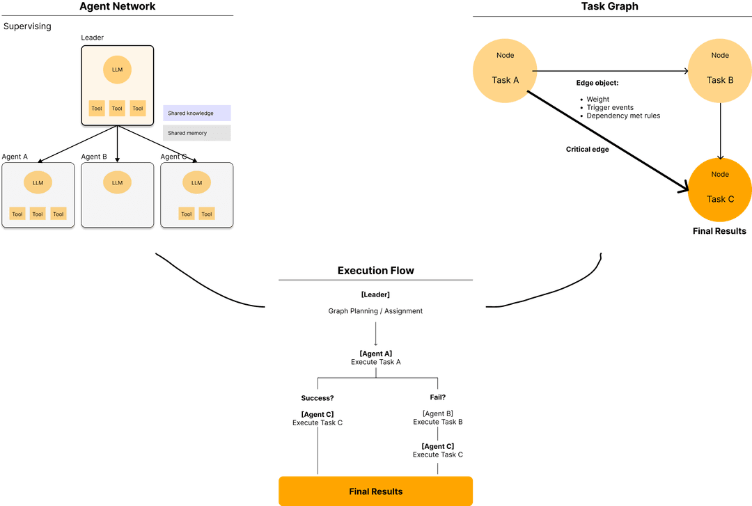
Key Features
versionhq is a Python framework designed for automating complex, multi-step tasks using autonomous agent networks.
Users can either configure their agents and network manually or allow the system to automatically manage the process based on provided task goals.
Agent Network
When multiple agents handle a task, agents will adapt to specific network formation based on the task and network complexity.
You can specify a desired formation or allow the leader to determine it autonomously (default).
| Solo Agent | Supervising | Squad | Random | |
|---|---|---|---|---|
| Formation | 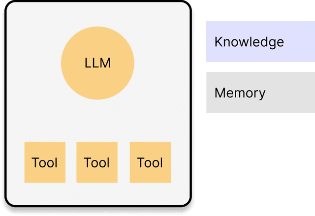 | 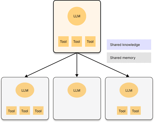 | 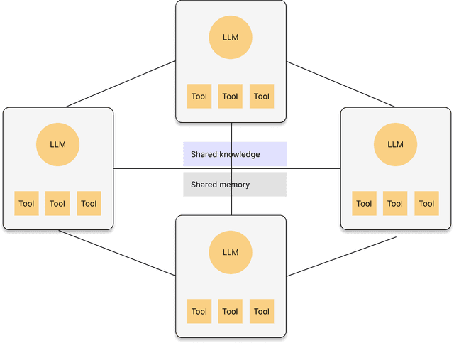 | 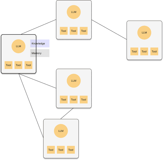 |
| Usage |
|
|
|
|
| Use case | An email agent drafts promo message for the given audience. | The leader agent strategizes an outbound campaign plan and assigns components such as media mix or message creation to subordinate agents. | An email agent and social media agent share the product knowledge and deploy multi-channel outbound campaign. | 1. An email agent drafts promo message for the given audience, asking insights on tones from other email agents which oversee other clusters. 2. An agent calls the external agent to deploy the campaign. |
Kuriko Iwai
Kernel Labs Pte. Ltd.
Kuriko Iwai
Shipping AI Systems?
I help teams design and deploy scalable ML / RAG / LLM pipelines and MLOps infrastructure.
Or explore:
- Dive deeper 👉 Research Archive
- Learn by building 👉 AI Engineering Masterclass
- Try it live 👉 Playground
Related Books
These books cover the wide range of ML theories and practices from fundamentals to PhD level.

Linear Algebra Done Right

Foundations of Machine Learning, second edition (Adaptive Computation and Machine Learning series)

Designing Data-Intensive Applications: The Big Ideas Behind Reliable, Scalable, and Maintainable Systems

Machine Learning Design Patterns: Solutions to Common Challenges in Data Preparation, Model Building, and MLOps