Fixing Selection Bias in Enterprise Data with Inverse Propensity Scoring (IPS)

[Series] Causal Machine Learning - 2. De-Biasing Historical Data Logs (without Expensive A/B Tests)

By Kuriko IWAI

Table of Contents

In Part 1, we explored the feature flattening trap of standard machine learning (ML) models and how causal inference can guide business strategy.

But knowing a trap exists doesn’t fix our data - to rewrite the biased historical data, we have to deal with selection biases.

Inverse Propensity Scoring (IPS) provides a solution to this challenge by re-weighting historical observational logs to synthetically simulate a Randomized Controlled Trial (RCT).

This article explores the mechanics and vital role of IPS through a case study of an engineering organization facing challenges with project allocation and employee retention.

◼ The Use Case - Project Routing Dilemma

To ground our solution, let us establish the core challenge we are trying to solve across a large engineering organization.

Imagine the organization is transitioning from legacy, manager-driven project routing to an automated, causal-AI driven engine designed to maximize 1-year developer retention.

▫ Confounded Project Routing with Selection Bias

Let's say, human managers preferred engineers from top-tier universities when assigning to Tier-1 projects.

On the other hand, they route engineers from non-traditional backgrounds mostly to standard, legacy maintenance work.

Because Tier-1 projects tend to have more visibility and learning opportunities, the elite cohort is systematically routed to high-success environments where they are pre-selected to succeed.

In this scenario, the historical logs are deeply poisoned by selection bias (right):

Figure A. Causal DAG diagram illustrating selection bias. X is confounder like an engineer's educational background, Y is the final outcome like 1-year retention, Z is the intervention like project assignments.

And if we pipe this raw data into standard ML, the model will inherently mistake an engineer's educational background for the project's inherent value.

To break this loop, we must understand how different study designs capture this data—and why Inverse Propensity Scoring (IPS) is needed to synthetically fix it.

The absolute cleanest way to solve our project routing dilemma is a Randomized Controlled Trial (RCT).

An RCT is a scientific experiment where baseline biases are eliminated by design using a perfectly random allocation mechanism.

◼ Core Mechanism

Below diagram illustrates its mechanism:

Figure B. Workflow diagram of a Randomized Control Trial (RCT) showing candidate pool randomization into balanced treatment and control groups (Created by Kuriko IWAI).

In an RCT, a pool of subjects is split into a treatment group (A_0 = 1) and a control group (A_0 = 0), following:

• Control Group: A baseline group that receives no intervention (e.g., keeping developers on standard maintenance).

• Randomization: Allocation is completely randomized. All potential baseline biases—whether they stem from a candidate's university pedigree, years of experience, or technical stack—are distributed evenly across both groups.

• Blinding: To further mitigate psychological or observer biases, subjects (single-blind) or both subjects and researchers (double-blind) are kept unaware of group assignments.

By balancing these baseline traits perfectly, RCTs provide the surest means of achieving two critical benchmarks of research quality:

• Internal Validity: Ensuring that the relationships found within the study data reflect true, unconfounded causal relationships in the target population.

• External Validity: Ensuring that the results calculated by the model can be confidently applied to similar populations in different real-world settings.

◼ Applied to the Use Case: The Live Hiring RCT

If we ran a pristine RCT in our engineering org, we would take a fresh pool of 1,000 incoming developers.

Regardless of whether they went to an Ivy League university or a self-paced coding bootcamp, we would flip a coin:

• Heads (A_0 = 1) → Sent directly to a Tier-1 Cloud Architecture project.

• Tails (A_0 = 0) → Sent directly to standard maintenance.

Because both groups are structurally identical at day zero, any variance in our final 1-year retention outcome (Y) could be confidently attributed to the project assignment (A_0) alone.

While the live hiring RCT yields perfectly clean data, running it in a production environment hits an immediate operational wall.

◼ Why Live Hiring Experiments Fail Operationally

There are two main reasons that the experiment fails in production:

1. Severe operational risk and

2. Ethical constraints.

▫ 1. Severe Operational Risk and Costs

Forcing a randomized assignment policy is hazardous.

If we randomly assign an under-qualified team to a critical tier-1 infrastructure project just to gather unconfounded data, we'd risk catastrophic downtime and lost revenues.

▫ 2. Ethical Constraints

It can be highly disruptive to intentionally strip career-advancing, beneficial treatments like premier projects away from a control group simply to satisfy an algorithmic requirement.

◼ Alternative Analytical Studies

Because of these operational frictions, we must pivot to alternative study designs.

The below diagram shows the breakdown of analytical study designs:

Figure C. Taxonomy chart of analytical study designs categorizing experimental variants and observational frameworks like cohort, case-control, and cross-sectional studies.

▫ A. Experimental Variants

• Non-Randomized Controlled Trials: We actively manipulate the assignment policy, but rely on non-random criteria (like team tenure or hiring dates) to form groups.

  • Use Case Example: We roll out an automated Tier-1 project routing pilot exclusively to our Tokyo office, while keeping our New York office on legacy manager routing.

  • The Causal Flaw: Without a random coin flip, the baseline traits ($X$) of the Tokyo engineering culture differ systemically from New York, leaving the door open for hidden regional confounders.

▫ B. Observational Frameworks

When we cannot manipulate project assignments at all, groups form naturally in historical operational logs.

• Cohort Studies: 

  • Isolates a group of developers right at their hire date, record their initial baseline context, and actively follow them forward over a 12-month period.

  • Use Case Example: Tracking developers as they naturally land Tier-1 projects or standard maintenance based on legacy human manager preferences.

• Case-Control Studies: 

  • Instead of waiting 12 months, identifies two terminal groups: the “Cases” (developers who left the company within 1 year) and the “Controls” (developers who stayed). We then analyze their past logs to check what project exposures and baseline traits drove the split.

  • Use Case Example: This is a massive time-saver for studying rare infrastructure failures or extreme corporate attrition, though we must heavily adjust for survivorship bias.

• Cross-Sectional Studies (Snapshots): 

  • Measures exposure and outcomes at the exact same time.

  • Use Case Example: Pulling a data dump of our entire global directory today to see which developers are currently on Tier-1 projects and matching that to their current Q3 happiness score. It provides a quick operational snapshot but cannot establish a clear chronological sequence of events.

▫ Comparing RCTs and Observational Alternatives

To see exactly how these choices impact our causal pipeline, let us map our project routing challenge across these methodologies:

Table 1. Methodological Trade-offs: Randomized Experiments vs. Observational Cohorts

Because running RCT in our use case is operationally too risky, we must debias our historical data logs synthetically.

Inverse Propensity Scoring (IPS) is a causal inference framework designed to estimate the true causal effect of an action when running a live RCT is impractical.

The below diagram illustrates its core concept:

Figure D. Distribution graph demonstrating how Inverse Propensity Scoring (IPS) re-weights skewed observational data into a balanced synthetic sample (Created by Kuriko IWAI)

Figure D shows that IPS can synthetically adjust the balances by re-weighting the original population with selection biases.

In our use case, when an Ivy League graduate (red circles, Figure D) had a 95% chance of being selected for a Tier-1 project based on their pedigree, their data point is down-weighted (IPW = 1.05 < 20).

Conversely, if an equally capable engineer from a non-traditional background (orange circle, Figure D) was selected for a Tier-1 project against all historical odds (a 5% probability in reality), their data point is up-weighted by a factor of 20 (IPW = 20).

This synthetic adjustment balances the distribution of baseline confounder X to look statistically identical across both groups.

◼ The Exchangeability of IPS

The exchangeability of IPS indicates its ability to transform a biased historical log into a clean, pseudo population where treatment and control groups can be fairly compared without risking live revenues.

This is critical to causal inference.

Causal inference attempts to answer prescriptive questions such as:

"What will happen to our retention rate if we change our active policy and assign this specific cohort to a Tier-1 project?",

But in reality, causal inference faces counterfactuals where it cannot observe what would happen when Engineer A were assigned to the control group (A_0 = 0), and vice versa.

So, without IPS, causal inference collapses because confounding (high-performing profile) simultaneously causes a higher likelihood of being assigned to the treatment group (A_0 = 1), and can naturally exhibit higher retention (Y).

1                  [Confounder: Engineer with Pedigree (X)]
2                                 /          \
3                                /            \
4                               v              v
5[Project Assignment (A0)] ----------> [1-Year Retention (Y)]
6

Figure E. Causal loop diagram showing baseline confounder X directly influencing both the treatment action A_0 and the retention outcome Y, resulting in entangled correlation and causation (Created by Kuriko IWAI)

IPS can mathematically strip away this dilemma.

To understand how IPS achieves synthetic randomization, let us look at the underlying mathematical framework.

◼ Core Variables

IPS has three key variables:

• X: Baseline confounder. A vector of observed baseline confounders. In the hiring context, X can be a jobseeker's professional background.

• A_0 ∈ {0, 1}: An intervention. The binary treatment indicator represents the primary initial action. For instance, A_0 = 1 if assigned to a complex Tier-1 project, A_0 = 0 if assigned to standard maintenance.

• Y: The target outcome. For instance, retention status or promotion after 1 year. Y(1), Y(0 indicate the potential outcomes (counterfactuals) if the jobseeker were un/treated by the intervention A_0 (e.g., assigned a complex project), respectively.

◼ Propensity Score

The propensity score e(X) is the conditional probability of receiving the treatment given the baseline confounder X:

where A_0 = 1 represents that an individual (jobseeker) is assigned to an intervention A_0.

In an enterprise ML pipeline, this score is typically estimated using a calibrated binary classifier such as Logistic Regression or LightGBM trained on historical logs to predict A_0 from X.

◼ Estimating IPS

To isolate the true structural impact of our action, the Average Treatment Effect (ATE) can measure the average total causal impact of the policy change across the entire population.

Mathematically, ATE is denoted:

Here, E[Y(1)] is the expected value of the outcome if every single individual in the population had been forced into the treatment group (A_0 = 1).

In the hiring context, this represents a situation where all jobseekers (employees) are assigned to the competitive project A_0 = 1 for instance.

On the other hand, E[Y(0)] is the expected value of the outcome when A_0 = 0, meaning all jobseekers are assigned to a simple, baseline project.

Because we can never simultaneously observe both Y(1) and Y(0) for a single individual, the IPS estimator allows us to calculate these unobserved counterfactual expectations using only observed data by applying Horvitz-Thompson inverse weights:

Where:

• A_0 ∈ {0, 1} is the observed treatment assignment for a given individual.

• Y is the actual observed outcome.

• e(X) is the estimated propensity score for that individual.

• A_0⋅Y / e(X) zero-out anyone who did not receive the treatment (A_0 = 0) and dynamically amplifies the outcomes of individuals who received the treatment despite a low historical probability.

◼ Computing Causal Weight

To operationalize this, the IPS pipeline computes an individual causal weight (w_i) for every single data point in our cohort:

For example:

For Engineer A: Ivy League Grad, 5 YOE

• Because managers actively favor this profile for top tasks, their estimated propensity score is highly skewed: e(X_A) = 0.95.

• They were assigned a Tier-1 project (A_A = 1).

For Engineer B: Non-traditional background, 1 YOE

• Because managers usually bypass this profile, their propensity score is low: e(X_B) = 0.05.

• Due to an emergency staff shortage, they were assigned a Tier-1 project anyway (A_B = 1).

Eq. 1.4 proves that the causal weight for Engineer A remains almost one:

while Engineer B's data point is scaled up by a factor of 20:

As Figure D shows, this re-weighting can evenly distribute population to the treatment and control group in the pseudo-population.

▫ Defining Selection Bias in Math

In the original historical logs, the conditional probability of seeing a specific profile X with a specific project assignment A_0 is governed by the standard product rule of probability:

Because human managers prefer certain backgrounds, the assignment probability P(X, A_0) changes drastically depending on X.

As we saw in the previous example,

• For Engineer A, P(A_0 = 1 | X) = 0.95.

• For Engineer B, P(A_0 = 1 | X) = 0.05.

Selection bias indicates that the confounder X and treatments A_0 are statistically dependent.

▫ Mitigating Selection Bias

Securing statistic independence between the confounder X and treatments A_0 can mitigate selection biases.

Let's look closely at how Eq 1.4 treats a person who actually received the treatment (A_i = 1).

For anyone in the treatment group, the second half of Eq 1.4 drops out because (1 - A_i) = 0.

Their individual weight simplifies to:

Now, let's observe what happens when we create a pseudo-population by multiplying our original observational probability distribution P(X, A_0=1) by this exact mathematical weight:

Substitute the definitions from Eq 2.1 and Eq 1.4 into this equation:

▫

By running the exact same math for the control group (A_0 = 0) and combine both branches back together, the new, synthetically weighted joint distribution of the dataset simplifies to:

Eq. 2.3 forces X and A_0 to become independent; the baseline features balance perfectly across both treatment branches.

This converts the heavily skewed observational logs into a clean synthetic sandbox.

Let’s implement this de-biasing pipeline in Python.

We will simulate a confounded corporate dataset where legacy managers over-indexed on an employee’s technical background (X) when assigning them to Tier-1 projects (T).

We will showcase how a standard model overestimates the impact of the project assignment, and how our IPS pipeline recovers the ground truth.

1import numpy as np
2import pandas as pd
3import sklearn.linear_model as lm
4import statsmodels.api as sm
5import statsmodels.formula.api as smf
6
7# simulate a dataset with a confounder (X), treatment assignment (A_0), and outcome (Y)
8np.random.seed(42)
9N = 12000
10
11X = np.random.normal(0, 1, N)
12
13prob_A = 1 / (1 + np.exp(- (1.8 * X)))
14A_0 = np.random.binomial(1, prob_A)
15
16
17true_beta_A0 = 0.6
18prob_Y = 1 / (1 + np.exp(- (-1.0 + true_beta_A0 * A_0 + 1.2 * X)))
19Y = np.random.binomial(1, prob_Y)
20
21df = pd.DataFrame({'X': X, 'A_0': A_0, 'Y': Y})
22
23# native estimation of the effect of A_0 on Y without any adjustment for confounding
24naive_model = smf.logit("Y ~ A_0", data=df).fit(disp=0)
25naive_beta = naive_model.params['A_0']
26
27# ips pipeline - estimating propensity scores using logistic regression
28propensity_model = lm.LogisticRegression(penalty=None)
29propensity_model.fit(df[['X']], df['A_0'])
30df['propensity_score'] = propensity_model.predict_proba(df[['X']])[:, 1]
31
32# check positivity violation: propensity scores should be bounded away from 0 and 1
33min_score, max_score = df['propensity_score'].min(), df['propensity_score'].max()
34print(f"Propensity Score Range: [{min_score:.4f}, {max_score:.4f}]")
35
36# compute ipw
37df['weight'] = df['A_0'] / df['propensity_score'] + (1 - df['A_0']) / (1 - df['propensity_score'])
38df['id'] = df.index
39
40# fit a GEE model to estimate the causal effect of A_0 on Y using the computed weights
41ips_model = smf.gee(
42    "Y ~ A_0", 
43    groups="id", 
44    data=df, 
45    family=sm.families.Binomial(link=sm.families.links.Logit()), 
46    weights=df['weight']
47).fit()
48ips_beta = ips_model.params['A_0']
49
50

◼ Results

▫ Propensity Score Range: [0.0011, 0.9990]

The score range shows the lowest and highest probabilities the model calculated for a developer getting assigned to a Tier-1 project.

The range is incredibly extreme from almost zero to 1; a score of 0.0011 means a developer had a 0.11% chance of getting a Tier-1 project but got it anyway, while 0.9990 means they had a 99.9% chance.

This tells us that management's selection bias was extremely severe, creating a massive imbalance in who got selected for top projects.

▫ Intervention (treatment assignment) A_0

1. The ground truth: A_0 = 0.60

This indicates the actual, unconfounded impact of a Tier-1 project assignment to 1-year retention Y.

In a perfect world like a clean RCT experiment, giving a developer a Tier-1 project increases their baseline retention metrics by exactly 0.60.

This is the benchmark number the causal model is trying to find.

2. Naive observation by standard ML (logistic regression): A_0 = 1.6974

This is what a standard ML model sees if we just feed it raw historical data without correcting any biases.

The number is massively inflated (1.6947 vs the true 0.60).

Because managers historically gave Tier-1 projects to the highest-performing engineers, a standard model incorrectly credits the project for high retention, when in reality, those elite engineers were already highly likely to stay regardless of their assignment.

3. IPS re-weighted causal inference: A_0 = 0.4415

This is the calculation from the corrected causal inference pipeline after using IPS to strip away historical management bias.

It successfully broke the bias, moving drastically closer to the real-world truth of 0.60.

Note: It is slightly lower than 0.60 because of the extreme probability weights we saw in step 1, which introduce statistical noise, and because of how math behaves when dealing with log-odds binary outcomes.

While IPS is mathematically competitive, its real-world deployment faces a roadblock: the positivity violation.

Formally, the IPS math requires to secure non-zero probabilities

for every unique combination of baseline confounders X.

This indicates that all individuals in the original population must land in either the treatment or control group.

▫ Hitting the Wall: Strict Corporate Rules

But is it realistic?

Imagine our engineering organization in the use case enforces a rigid corporate rule:

When the propensity model evaluates this junior subpopulation X_{junior}, the historical probability of treatment drops to absolute zero:

due to the new rule.

So, when the IPS pipeline attempts to calculate the counterfactual expectation for the treatment group, the denominator in the formula collapses:

making it impossible to run causal estimation.

As Eq. 3.3 shows, when a subpopulation has a probability of exactly 0 or 1, IPS fails completely.

In other words, no optimization and tuning efforts can recover a causal signal from an environment where alternative actions were never attempted.

One cannot simulate the strategy because we have zero historical data points to balance.

◼ How to Overcome the Positivity Violation in Production

When hitting a deterministic corporate policy, we'd deploy two primary mitigation strategies to save the pipeline:

▫ Option 1. Trimming and Restricting the Causal Manifold

The most pragmatic engineering solution is to redefine the scope of your causal inquiry.

If e(X_{junior}) = 0, we must explicitly remove junior engineers from the model's dataset entirely - and include only mid-level and senior engineers where true managerial discretion exists (0 < e(X) < 1).

This allows the model to regain mathematical stability, but we sacrifice scope.

"We can optimize routing for experienced engineers, but we cannot mathematically evaluate counterfactuals for junior engineers because alternative choices were never attempted."

▫ Option 2. Utilizing Dynamic Overlap via System Shocks (Natural Experiment)

If historical exceptions exist that break the rigid corporate rule, we can use them as counterfactual data whose e(X) > 0 is secured.

For example, a massive cloud outage occurred last quarter forced managers to temporarily pull junior engineers onto Tier-1 response teams.

This can be used to calculate valid weights for junior engineers.

By applying IPS, we successfully forced our historical log data to simulate an unbiased, randomized experiment.

We decouple an engineer's entry-level background from the true, isolated impact of their project placement.

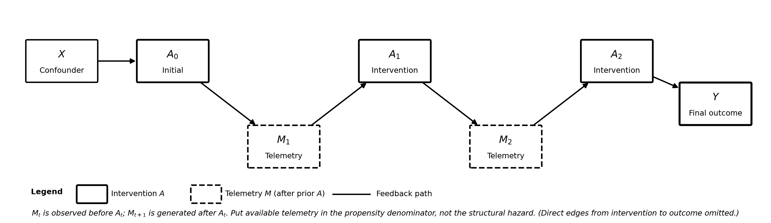
But this brings us to the ultimate caveat of IPS: IPS is a static snapshot game.

◼ The Time Varying Trap

IPS assumes all baseline traits X are measured at day one, and the intervention A_0 is a single, permanent choice.

But in reality, corporate environments are continuous, evolving timelines.

Consider this common production feedback loop:

1. A junior engineer is hired.

2. At Month 3, they perform exceptionally well on a small task (time-varying confounder).

3. Because of this success, the manager overrides standard policy and promotes them early to a Tier-1 team (time-varying treatment).

4. Their performance at Month 6 dictates their final 1-year retention Y = 1.

When past treatments affect future confounders, standard static IPS is completely blindfolded.

To solve this challenge, I'll explore Time-Varying Confounding and the Descent into G-Estimation in Part 3.

◼ Causal Machine Learning Series

• Part 1. Why Machine Learning Demands Causal Inference - Rethinking the Predictive Paradigm

• Part 2. De-Biasing Historical Data Logs (without Expensive A/B Tests)

Written by Kuriko IWAI. All images, unless otherwise noted, are by the author. All experimentations on this blog utilize synthetic or licensed data.

FAQ

Share What You Learned

Continue Your Learning

If you enjoyed this blog, these related entries will complete the picture:

• Why Machine Learning Demands Causal Inference

  

  Eliminate selection bias and structural confounding. Learn do-operator, graph surgery, backdoor criterion.

Related Books for Further Understanding

These books cover the wide range of theories and practices; from fundamentals to PhD level.

Linear Algebra Done Right

Foundations of Machine Learning, second edition (Adaptive Computation and Machine Learning series)

Designing Data-Intensive Applications: The Big Ideas Behind Reliable, Scalable, and Maintainable Systems

Machine Learning Design Patterns: Solutions to Common Challenges in Data Preparation, Model Building, and MLOps

Hands-On Large Language Models: Language Understanding and Generation