Deploy the inference via an API as a microservice.
The Project Kit
The ML Pipeline
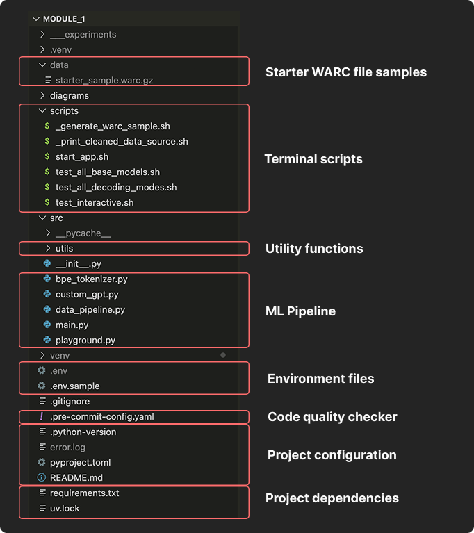
A modular Python codebase structured for readability and scalability:
The Data Architect:A custom pipeline for heuristic filtering and fuzzy deduplication of raw web data (Common Crawl).
The Vocabulary Logic: A Byte Pair Encoding (BPE) tokenizer implementation with custom vocabulary mapping.
The Inference Backbone: A GPT-style engine featuring manual implementations of:
Logits Management: Raw score generation.
The Sampling Layer: Controllable Temperature, Top-k, and Top-p (nucleus) logic.
Advanced Decoding: Fast Greedy Search vs. high-quality Beam Search strategies.
The Full-Stack Core System
An entire system to run the ML pipeline to serve downstream services:
Server: A FastAPI server ready for deployment with Pydantic schemas for the API.
Visual Playground: A Streamlit frontend with real-time sliders to visualize how parameters change AI behavior.
Pre-Commit Quality Hooks: Automated Git scripts that run linting, formatting (Black/Ruff), and syntax checks before every commit.
Dependency Management: Ready to use UV and pip for the dependency management.
Portfolio-Ready Documentation
README.md: A professional project overview including architecture diagrams, installation guides, and How It Works section designed to showcase your technical depth on GitHub.
Project Manifest: A clear breakdown of the system design and tech stack (Python, PyTorch, FastAPI).
Quick-Start Experiment Kit
Starter Dataset: A curated sample of refined web data so you can run the pipeline immediately without waiting for a 1TB download.
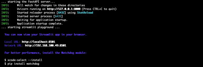
One-Command Setup: A start_app.sh script to handle virtual environment creation and dependency injection in seconds.
1chmod +x scripts/start_app.sh && uv run scripts/start_app.sh
Tutorial Summary
Instant access to the private GitHub repo and sample datasets 👇
The Project Kit
The ML Pipeline
A modular Python codebase structured for readability and scalability:
The Data Architect:A custom pipeline for heuristic filtering and fuzzy deduplication of raw web data (Common Crawl).
The Vocabulary Logic: A Byte Pair Encoding (BPE) tokenizer implementation with custom vocabulary mapping.
The Inference Backbone: A GPT-style engine featuring manual implementations of:
Logits Management: Raw score generation.
The Sampling Layer: Controllable Temperature, Top-k, and Top-p (nucleus) logic.
Advanced Decoding: Fast Greedy Search vs. high-quality Beam Search strategies.
The Full-Stack Core System
An entire system to run the ML pipeline to serve downstream services:
Server: A FastAPI server ready for deployment with Pydantic schemas for the API.
Visual Playground: A Streamlit frontend with real-time sliders to visualize how parameters change AI behavior.
Pre-Commit Quality Hooks: Automated Git scripts that run linting, formatting (Black/Ruff), and syntax checks before every commit.
Dependency Management: Ready to use UV and pip for the dependency management.
Portfolio-Ready Documentation
README.md: A professional project overview including architecture diagrams, installation guides, and How It Works section designed to showcase your technical depth on GitHub.
Project Manifest: A clear breakdown of the system design and tech stack (Python, PyTorch, FastAPI).
Quick-Start Experiment Kit
Starter Dataset: A curated sample of refined web data so you can run the pipeline immediately without waiting for a 1TB download.
One-Command Setup: A start_app.sh script to handle virtual environment creation and dependency injection in seconds.
1chmod +x scripts/start_app.sh && uv run scripts/start_app.sh
Instant access to the private GitHub repo and sample datasets 👇
In this project, we’ll implement a RAG framework for reasoning tasks, using pre-trained weights to summarize information retrieved from unstructured web-crawled data and WARC archives.
Below diagram illustrates how the entire workflows:
Kernel Labs | Kuriko IWAI | kuriko-iwai.com
Figure A. The system workflow (Created by Kuriko IWAI)
The workflow begins when a user submits a query and an HTML reference via the Streamlit interface.
The backend, powered by FastAPI, extracts and structures the raw text into a prompt for the model.
Then, the system utilizes a custom BPE tokenizer (orange boxes) to process the user query and crawled data, feeding them into a uniquely configured GPT-based model (green box).
The model then performs an autoregressive process to generate a response by predicting subsequent tokens.
Finally, the BPE tokenizer decodes these tokens into human-readable text for the user.
◼ WARC for High-Signal Extraction
Among Common Crawl’s three primary file formats in Figure A, WET (extracted text) is the most frequently used for LLM training because processing raw WARC/HTML files at scale is an operational burden.
While WAT provides richer metadata, including HTML tags and link structures, WET is preferred for its pure textual format.
Although WARC is rarely used for standard LLM training due to its massive storage footprint, it remains invaluable for multimodal datasets.
We’ll opt for WARC in this project to implement custom filters and recover high-signal data discarded during the standard WET extraction process.
Data Curation & Preprocessing
Before a model can reason, it must be trained on massive high-quality data to learn patterns applicable to next token predictions.
To demonstrate how data is ingested, we'll use a hybrid approach where the system performs a web crawl to extract real-time data, while referencing pre-trained vocabularies to ensure the model generates meaningful output.
This process consists of the following steps:
Raw web crawl: Extracts raw text data from targeted websites.
Heuristic filtering: Filters out low-quality content like non-natural language and isolated code fragments.
Deduplication: Identifies and consolidates duplicate content across different sources.
Tokenization: Maps the text data into tokens, implementing byte-level tokenization from scratch.
◼ Data Pipeline Engineering
To engineer data pipelines, we’ll leverage web crawling.
cWeb crawling can be performed either manually or systematically.
▫ Raw Web Crawls (Manual Crawl)
The most intuitive approach is a manual crawl, which involves accessing a website directly via its URL.
In this mode, the crawler functions like a standard web browser:
Request: It pings a specific, live URL.
Latency: It waits for the server to respond before proceeding.
Single-threaded: It processes only one site at a time.
Dynamic: Because it targets live sites, the data retrieved changes if the website is updated or goes offline.
▫ Common Crawl
Common Crawl, on the other hand, functions as a massive, historical archive like a snapshot of the entire internet, rather than browsing the live web. It is the standard of training for LLMs like GPT.
Compared to manual crawling:
No live requests: The system downloads large data files (WARCs) from Common Crawl, which contain pre-scraped data from thousands of sites.
High velocity: Data processing is limited only by the hardware's CPU/GPU speed, entirely bypassing the bottlenecks of internet latency and connection stability.
Massive throughput: Ingest thousands of websites simultaneously by reading compressed files rather than scraping URLs one by one.
To perform the common crawl, the system streams content from the WARC file to generate a continuous response:
1from warcio.archiveiterator import ArchiveIterator
23withopen(warc_file_path,'rb')as stream:4 records = ArchiveIterator(stream)5for record in records:6if record.rec_type =='response':7# decompress the payload8 raw_payload = record.content_stream().read()910# convert bytes to string (UTF-8)11 raw_html = raw_payload.decode('utf-8', errors='replace')12yield raw_html
13
◼ Heuristic Filtering
In the context of LLMs, heuristic filtering refers to the process of using rule-based curation of training data, removing low-quality, repetitive, or irrelevant content.
Because LLMs rely on massive datasets to master language, noisy data is captured by default. Training on such unfiltered data leads to several critical issues:
Hallucinations: Learns and reproduces incorrect patterns.
Bias and toxicity: Adopts harmful language or societal prejudices found in the raw text.
Computational waste: Low-value data costs expensive processing power.
Heuristic filtering ensures that the model learns only from high-quality human language.
Common techniques include:
Language distribution: Filters out pages with a low ratio of alphabetic characters (e.g., raw CSS code or random symbols).
Keyword & blocklist filtering: Removes documents that contain excessive toxic language or placeholders.
Repetition checks: Eliminates bot-like content where phrases are repeated unnaturally.
Length constraints: Discards snippets that are too short to provide context or excessively long data dumps.
Quality scoring: Uses metrics like the gunning-fog index or perplexity scores to ensure the text is readable and grammatically coherent.
In this project, we’ll simply remove irrelevant contents:
HTML tags.
Citations.
A line longer than twenty (20) characters.
Codes containing over three special characters.
◼ Deduplication
Deduplication is the process of removing redundant or near-identical data from a training dataset.
Specific content like boilerplate code or syndicated news articles frequently appears thousands of times in the training data.
Deduplication eliminates this redundancy to ensure the model learns from a diverse range of information, enabling the model to:
Reduce memorization: Avoid regurgitating verbatim text like privacy policies or copyrights.
Prevent bias: Prevent the model from misinterpreting the biased contents reposted across many websites as the ground truth.
Improve training efficiency: Shrink datasets up to 70%, reducing the computational cost.
Deduplication occurs at two primary levels:
Exact match: Removes text identical character-for-character.
Near-duplicate match: Uses algorithms like MinHash or Locality-Sensitive Hashing (LSH) to identify documents nearly identical (e.g., 90% similarity) but contain minor variations like different timestamps or formatting changes.
Technically, using a hash for deduplication is a standard practice for speed and memory optimization because comparing raw text strings directly requires enormous patterns of comparisons.
We’ll implement exact-match deduplication by checking the line's hash and skipping further processing if the hash already exists in our index:
After cleaning the raw text data, the tokenizer maps the text data into tokens.
Tokenizers can be categorized into three groups:
Word-based,
Character-based, and
Subword-based.
In this project, we’ll use a BPE tokenizer, an industry-standard, subword-based tokenizer used by GPT and Llama families.
BPE tokenizers take five technical steps:
Step 1. Byte-level mapping
Step 2. Preprocessing,
Step 3. Initial tokenization,
Step 4. BPE-merge operation, and
Step 5. Iteration
▫ Step 1. Byte-Level Mapping
First, the tokenizer maps all 256 possible raw bytes like 0x00, 0x0A to Unicode characters.
This prevents the raw bytes from breaking text-processing later on.
▫ Step 2. Preprocessing
Then, the text is split into manageable chunks using a regex pattern to isolate suffixes, contractions, and punctuation.
1import re
23# split text using gpt-2 regex pattern4pat = re.compile(r"'s|'t|'re|'ve|'m|'ll|'d| ?\w+| ?[^\s\w]+|\s+(?!\S)|\s+")5
This process ensures that the tokenizer does not merge characters across word boundaries.
For example, for the sentence “hello world“, the tokenizer cannot merge o and w because they belong to separate subwords.
▫ Step 3. Initial Tokenization
Then, the BEP tokenizer tokenizes the split data and creates adjacent pairs of tokens, while counting how many times each pair appears in the data (e.g., how many times "h" is followed by "e").
1# counts frequency of adjacent character pairs2pairs = collections.defaultdict(int)3# e.g., "hello" -> {('h','e'): 1, ('e','l'): 1, ('l','l'): 1, ('l','o'): 1}4
The resulting pairs and their rankings based on the count are stored in a merge table, a global list of priorities learned from a massive training dataset.
▫ Step 4. BPE-Merge Operation
Based on the merge table, the tokenizer identifies the most frequent pair among all created in Step 2:
1import requests
23lines = learned_merge_table.split('\n')[1:-1]4merges =[tuple(line.split())for line in lines]5bpe_ranks =dict(zip(merges,range(len(merges))))67# find the pair to be merged based on the learned priority8bigram =min(pairs, key=lambda pair: bpe_ranks.get(pair,float('inf')))9
The most frequent pair has the lowest index (hence, the highest merge rank) in the merge table.
The BPE tokenizer prioritizes the highest ranking pair to merge first.
For example:
Pair
Merge Rank
Merge Priority
('h', 'e')
5
Highest → Merge
('e', 'l')
42
Low
('q', 'z')
inf
Lowest → Never merge
Table 2. The merge table with merge priority (Created by Kuriko IWAI)
Once finding the pair to merge, it replaces every instance of the pair (e.g., ('h', 'e')) with a new, combined token (e.g., 'he') and records the merge in the merge table.
The implementation looks like:
1# retrieves the first and second highest priority pairs2first, second = bigram
34new_word =[]5i =06while i <len(word):7try:8# starting at the current index i, find the index that the same first pair occurs9 j = word.index(first, i)10# add all between the current index i and the found index j11 new_word.extend(word[i:j])12# move the next starting point to index j13 i = j
14except ValueError:15# the first pair is no longer in the list. add the rest and finish16 new_word.extend(word[i:])17break1819# check if the next token is the second priority pair20if word[i]== first and i <len(word)-1and word[i+1]== second:21# merge22 new_word.append(first + second)23 i +=224else:25 new_word.append(word[i])26 i +=127
Performance Note: Local caching can avoid redundant calculations during training:
This training process follows the original GPT-2 'merges.txt' priority logic to ensure compatibility with pre-trained weights.
Developer Note: During inference, fetching merges.txt will significantly slow down the system. So, LLMs use local versions of the pre-defined merges.txt file to avoid network calls.
▫ Step 5. Iteration Loop
The BPE tokenizer repeats Steps 2 and 3 until the vocabulary (initial 256 bytes + number of merges) reaches the target size (e.g., 50,257 for GPT-2).
In case of the word “hello“, the pair of ‘h‘ and ‘e‘ becomes a single unit 'he' in the next round, and the tokenizer might find 'he' + 'l' as the new most frequent pair in the following round.
1# the loop continues until we reach the target vocabulary size (50,257)2whilelen(vocab)< target_vocab_size:3 pairs = get_stats(word)4ifnot pairs:break56# identify the highest priority merge based on learned weights7 best =min(pairs, key=lambda p: bpe_ranks.get(p,float('inf')))8 word = merge(word, best)9
Performance Note: Although the merge table is global, the merge operation can only combine characters actually sitting next to each other in the subword. So, in the case of “hello“, “he” + “r” cannot be an option as “r“ is not right next to “he“ in “hello“.
Inference & Decoding Logic
Inference is the process and logic of generating the next token.
In this phase, we’ll:
Select base models,
Generate logits,
Implement decoding strategies, and
Apply autoregressive generation.
◼ Model Selection
To leverage the custom BPE tokenizer using GPT-2’s merge table, I’ll select following compatible models from the GPT family:
gpt2: The base model.
gpt2-medium / gpt2-large / gpt2-xl: The larger siblings of the base model.
distilgpt2: A smaller, faster version of the base model (CPU-friendly).
EleutherAI/gpt-neo-125M: An open-source replication of the GPT-3 architecture that follows the same causal logic.
Each model is loaded via the AutoModelForCausalLM class from the transformers library:
Logits are the raw, unnormalized numerical values (scores) generated by the final layer of the neural network for every token in the model’s vocabulary.
The scores represent the model's final insights on which token should come next before any probabilities are calculated.
Higher logit indicates that the model thinks the token is the correct continuation.
▫ Logits Bias
Optionally, we can manually adjust specific logits to make certain words more/less likely to appear in the output.
For example, to ban the word “Blue“ and encourages the word “Green“:
Another common way to modify the logits is using Temperature (T) that adjusts the sharpness of the distribution.
Below diagram demonstrates how temperatures modify the probability distribution:
Kernel Labs | Kuriko IWAI | kuriko-iwai.com
Figure B. Temperature scaling examples with T = 0.2, 0.7, 1.0 (original), 1.5, and 50 (Created by Kuriko IWAI)
At the original temperature (T=1.0, Colored orange in Figure B), the token 'sky' has a probability of 0.7; increasing T flattens the distribution, while decreasing T further sharpens it:
Lower T (<1) makes the distribution peakier. Favors high-probability words. Acts more deterministic.
Higher T (>1) flattens the distribution. Favors new words. Acts more creative and random.
We’ll apply the Temperature as the denominator of the logits:
Repetition Penalty is another way to adjust the logits by penalizing the probability of tokens that have already appeared in the text, forcing the model to explore a variety of words.
1rep_penalty =1.22input_ids = encoded_input.to(device)34for i inrange(input_ids.shape[0]):5# get unique tokens from the current sequence6 prev_tokens =set(input_ids[i].tolist())7for token_id in prev_tokens:8# apply penalty by decreasing/increasing logit if the value is positive/negative9if logits[i, token_id]>0:10 logits[i, token_id]/= rep_penalty
11else:12 logits[i, token_id]*= rep_penalty
13
▫ Probability Distribution
Lastly, the model applies the Softmax function to turn these logits into a probability distribution where all add up to 100%.
◼ Decoding Strategies
After the probability distribution is computed, the model applies decoding strategies to select the most appropriate next token from the candidate list, balancing coherence, creativity, and diversity.
In this project, we’ll set four base decoding strategies:
Greedy search,
Beam search,
Top-k sampling, and
Top-p (Nucleus) sampling
Below diagram compares each decoding method:
Kernel Labs | Kuriko IWAI | kuriko-iwai.com
Figure C. Comparing how each decoding method choose the next token (Created by Kuriko IWAI)
▫ Greedy Search
Greedy search is the simplest method where the model picks the token with the highest probability.
The beam width adjusts how many alternative sequences the model tracks, helping the model to find a sentence (rather than just a token) with globally higher-probability.
For example, when the beam width is two, the algorithm maintains the two most likely sequences (paths) at each step:
Kernel Labs | Kuriko IWAI | kuriko-iwai.com
Figure D. How Beam Search with beam width two selects the next token (Created by Kuriko IWAI)
The algorithm evaluates all possible next-token extensions for the current paths, keeps the two sequences with the highest combined probability, and discards the rest to save the computational cost.
▫ Top-k Sampling
Top-K sampling limits the selection to the top K most likely tokens, such as k=50.
Top-P (Nucleus) sampling selects the smallest set of tokens whose cumulative probability exceeds the threshold P such as p=0.9 (90%), allowing the model to expand candidate tokens based on the probability distribution.
Based on the probability distribution and the decoding strategy, the model continuously selects a single next token.
The custom BPE tokenizer decodes the newly-generated tokens to human-readable sentences:
1prompt_len = encoded_input.shape[1]23# retrieves the newly generated tokens4generated_tokens = input_ids[0][prompt_len:]56# decode7decoded_output = tokenizer.decode(generated_tokens)89# remove eos tags10final_output = decoded_output.replace('<|endoftext|>','').strip()11return final_output
12
▫ Developer Note:
Implementing Beam Search with tensor stacking is the most common point of failure for LLM backbones. If you want to skip the debugging and see the production-ready FastAPI implementation, you can download the Full-Stack Project Kit here.
The Inference Workflow
During inference, the tokenizer uses the merge table to ensure that the input is tokenized exactly the way the model saw it during training.
This process follows a four-step cycle:
Human: Type the word “The".
Tokenizer: Scans its merge table to see if "T" and "he" should be one unit. It decides “ The" is a single known entry and converts it to Token ID 464.
LLM: Receives the ID 464. Compute a probability distribution over its entire vocabulary using weights. Predicts the next most likely Token ID 345.
Tokenizer: Takes the ID 345, looks it up in its vocabulary (derived from the merge table), and translates it back into the human-readable string “ sunny".
Decoupling the merge table (vocabulary) from the LLM weights (meaning and logic) can enhance consistency and computational efficiency.
Consistency: LLMs can always receive data in the exact same token IDs it learned during training, preventing confusion.
Computational efficiency: LLMs can read much faster and process longer sentences because the merge table represents common subwords like "The" as a single ID.
Deployment
In the final phase, we’ll develop the infrastructure required for model deployment and accessibility.
The system comprises two main components:
FastAPI Microservice: A wrapper for the inference code that enables downstream services to submit prompts via JSON requests and receive real-time responses.
Streamlit Dashboard: An interactive interface allowing users to select base models and decoding strategies, fine-tune parameters via sliders, and input both data source URLs and specific queries.
This setup allows users to generate immediate responses and compare performance across various configurations.