Aligning LLMs with Direct Preference Optimization (DPO)

Learn the fundamentals and follow a technical walkthrough with Unsloth and Llama.

Machine LearningDeep LearningData SciencePythonLLM

By Kuriko IWAI

Introduction What is Direct Preference Optimization (DPO)

The Math Behind the Magic

KL-Regularization Coefficient

Comparing with Traditional RLHF

Major Use Cases of DPO

DPO in Action - Fine-Tuning Llama 3 with Unsloth

The Workflow

Step 1. Collecting Training Set

Step 2. SFT

Step 3. DPO

Wrapping Up

When to Stick with Traditional RLHF

References

Introduction

Training a Large Language Model (LLM) used to require two steps; first, predict the next word; next, rank its answers to fine-tune the behaviors.

This second part, known as Reinforcement Learning from Human Feedback (RLHF), has been the industry standard—but it’s complex and finicky.

Direct Preference Optimization (DPO) offers a streamlined alternative by framing the preference problem into a simple classification problem.

In this article, I’ll explore the fundamental mechanisms of DPO and apply it to the base model (Llama 3 8B) for a tone and style tuning task to demonstrate how it works in the LLM pipeline.

What is Direct Preference Optimization (DPO)

Direct Preference Optimization (DPO) is a technique to align the model with human preferences much simpler and more stable than the standard Reinforcement Learning from Human Feedback (RLHF).

The diagram below compares DPO with traditional RLHF:

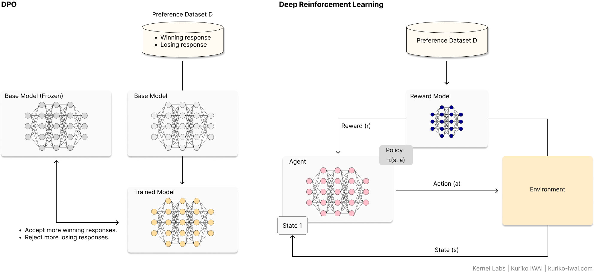
Figure A: Comparison diagram of DPO vs RLHF architectures showing preference dataset training and reward model loops (Created by Kuriko IWAI)

Initially introduced in a paper by Rafailo et al [1]., DPO (left, Figure A) trains the base model using the preference dataset D to accept more winning (preferred) responses, while rejecting more losing responses, than the base model.

For example, in a tone & style tuning task, when a user asks if they should head out for a walk:

A winning response can be: "It’ll probably start dumping rain this afternoon, so definitely grab an umbrella if you head out.", which sounds like a casual, helpful persona, while
A losing response can be: "There is a high probability of precipitation this afternoon. It is advisable to carry an umbrella.", which sounds like a robot.

DPO trains the base model to lean toward winning responses which align with human preference.

On the other hand, RLHF (right, Figure A) needs to run two computational heavy processes:

Training a reward model (neural network in black, right, Figure A) to score how good a response is based on human rankings.
Optimizing the policy by using reinforcement learning to nudge the model toward higher scores.

DPO can streamline these processes by removing the reward model from the system.

◼ The Math Behind the Magic

Instead of increasing a reward from the reward model, DPO attempts to directly increase the likelihood of the winning response, while decreasing the losing response.

Its objective function is mathematically denoted:

L_{DPO}(\pi_{\theta}; \pi_{ref}) = -\mathbb{E}{(x, y_w, y_l) \sim D} \left[ \log \sigma \left( \beta \log \frac{\pi{\theta}(y_w | x)}{\pi{ref}(y_w | x)} - \beta \log \frac{\pi_{\theta}(y_l | x)}{\pi_{ref}(y_l | x)} \right) \right] \quad \cdots \text{(1.1)}

Where:

πθ: The trained model.
π_ref: The base model (reference model).
x: The prompt (context or question) given to the model.
y_w, y_l: The winning and losing responses to the prompt x, all are pulled from the entire collection of human preferences D.
E(.): Expected losses across the entire collection D.
σ(): Sigmoid function:

\sigma(z) = \frac{1}{1 + e^{-z}} \quad \cdots \text{(1.2)}

β: A hyperparameter (KL-regularization coefficient) to penalize the trained model diverting from the base model. Industry standard: β = 0.1.

The subtraction in the DPO’s objective function Eq. 1.1 represents its preference strengths.

The first part of the subtraction measures how much more likely the trained model πθ makes the winning response y_w compared to the base model π_ref.

If this value is positive, the model is learning to prefer the winning answer.

So, DPO aims to increase this value.

The second part of the subtraction, on the other hand, measures how much the trained model πθ still prefers the losing response y_l compared to the base model π_ref.

DPO aims to decrease this value.

In consequence, the overall objective of DPO is to maximize the difference between these two by:

Increasing the probability of the winning response y_w, and
Decreasing the probability of the rejected response y_l.

◼ KL-Regularization Coefficient

The KL-regularization coefficient β is a hyperparameter which controls how much DPO penalizes the model for deviating from the base model π_ref.

The initial research by Rafailov et al.[1] found that β = 0.1 is the sweet spot for most general-purpose chat and instruction-following models.

But adjusting β can yield a response closer to or far away from the human preference:

Value Range	Characterization	Result
Low β ≤ 0.05	Aggressive	The model focuses heavily on following preferences. It can generate higher performance, but might result in model collapse or generate repetitive/unnatural responses as it drifts too far from the base model.
Mid 0.1 ≤ β ≤ 0.2	Balanced	The industry standard. Effectively learns human preferences while maintaining the linguistic quality and fluency of the base model.
High β > 0.5	Conservative	The model stays very close to the base model. It is very stable but may fail to learn human preferences.

Table 1: Impact of Hyperparameter β on Model Behavior and Stability.

It is common to adjust β based on specific goals:

Reasoning or coding: Use a lower β (e.g., β = 0.05) to force the model to strictly adhere to the preferred answer.
Creative writing: Use a slightly higher β (e.g., β = 0.2) to ensure the model doesn't lose its diverse vocabulary and style.
Small human preference dataset D: Use a higher β (e.g., β = 0.5) to prevent the model from over-fitting to a few noisy examples.

◼ Comparing with Traditional RLHF

Traditional RLHF can be unstable and computationally expensive because it needs to train a separate reward model, and then use complex algorithms like Proximal Policy Optimization (PPO).

As Figure A shows, the three key components; an agent, a reward model, and a value function must sync up well during training because when one moves too fast, the whole system crashes.

DPO achieves faster and more stable training primarily because:

Direct mapping: Redefines the alignment problem of the traditional RLHF as a simple classification problem denoted in Eq. 1.1.
Reduced overhead: No need to train or host a separate reward model, saving significant GPU memory.
Mathematical convergence: Avoids reward hacking where the model is stuck in a loophole attempting to get a high reward without actually returning a preferred response.

Here is the summary of the comparison:

Feature	Standard RLHF (PPO)	DPO
Complexity	High (Requires multiple models in memory)	Low (Just the policy and reference model)
Stability	Finicky (Sensitive to hyperparameters)	Stable (Essentially a supervised loss)
Efficiency	Slower and memory-intensive	Faster and more lightweight
Performance	Top-tier, but hard to achieve	Often matches or exceeds PPO in practice

Table 2: Architectural Comparison: Traditional RLHF (PPO) vs. DPO.

◼ Major Use Cases of DPO

Thanks to its stability and efficiency, DPO has become the go-to alternative of the standard RLHF.

Its use cases include:

Safety alignment: Reducing harmful, biased, or toxic outputs by training the model to prefer safe responses over unsafe ones.
Tone and style tuning: Shifting a model’s personality (e.g., making it more professional, witty, or empathetic) based on curated examples.
Summarization quality: Training models to prioritize summaries that are concise and factually accurate over those that are wordy or hallucinated.
Coding assistance: Teaching models to favor functional, bug-free code snippets over syntactically incorrect alternatives.
Reasoning and logic: Encouraging the model to choose step-by-step chain-of-thought explanations rather than jumping straight to a (potentially wrong) answer.
Instruction following: Improving the model's ability to strictly adhere to complex formatting or constraint-based prompts.

Developer Note - Bradley-Terry Model for DPO

DPO uses the Bradley-Terry (BT) model to transform the preference modeling problem into a classification loss function (Eq.1.1) to achieve the efficient training process.

The BT model defines the probability of a human preferring a winning response y_w over y_l using a reward function r(x, y):

P(y_w \succ y_l | x) = \sigma(r(x, y_w) - r(x, y_l)) \quad \cdots \text{(2.1)}

In standard RLHF, the optimal solution (π^*) that can maximize the reward r(x, y) is denoted:

r(x, y) = \beta \log \frac{\pi^*(y | x)}{\pi_{ref}(y | x)} + \beta \log Z(x) \quad \cdots \text{(2.2)}

where Z(x) is a partition function that ensures everything sums to 1.

Rafailo et al. decided to substitute the subtraction in Eq.2.1 with Eq.2.2 to cancel out the heavy computation of Z(x):

r(x, y_w) - r(x, y_l) = \left( \beta \log \frac{\pi(y_w | x)}{\pi_{ref}(y_w | x)} + \beta \log Z(x) \right) - \left( \beta \log \frac{\pi(y_l | x)}{\pi_{ref}(y_l | x)} + \beta \log Z(x) \right)

= \beta \log \frac{\pi(y_w | x)}{\pi_{ref}(y_w | x)} - \beta \log \frac{\pi(y_l | x)}{\pi_{ref}(y_l | x)} \quad \cdots \text(2.3)

Putting Eq.2.3 back to Eq.2.1:

P(y_w \succ y_l | x) = \sigma\Bigg(\beta \log \frac{\pi(y_w | x)}{\pi_{ref}(y_w | x)} - \beta \log \frac{\pi(y_l | x)}{\pi_{ref}(y_l | x)}\Bigg) \quad \cdots \text{(2.4)}

Eq. 2.4 represents the objective function of DPO (as shown in Eq.1), whose negative log-likelihood is minimized during the model training.

DPO in Action - Fine-Tuning Llama 3 with Unsloth

In this section, I'll tune the base model, Llama 3-8B with DPO for a tone and style tuning task.

◼ The Workflow

The workflow involves three main steps:

Step 1. Collecting training set.

Step 2. Supervised Fine-Tuning (SFT): Tune the base model (Llama 3 8B) with QLoRA.

Step 3. DPO training: Tune the trained model with DPO.

◼ Step 1. Collecting Training Set

The first step is to collect training data for SFT and DPO:

1 [
2  {
3    "prompt": "How are you liking that new setup you put together?",
4    "chosen": "I'm obsessed with this new mechanical keyboard, the switches feel like butter.",
5    "rejected": "The mechanical keyboard is functioning within expected parameters. The linear switches provide a smooth actuation force, which is often compared to a soft dairy product. I am pleased with the hardware."
6  },
7  {
8    "prompt": "How was that project sync today? Did it help clear things up?",
9    "chosen": "Honestly, the meeting could have been an email. I'm just tired of the bloat.",
10    "rejected": "The meeting was unproductive as the information shared did not require real-time synchronization. Corporate inefficiency often leads to time-management challenges. I acknowledge your dissatisfaction."
11  }
12]
13

I'll use the same data source for both and redefine the dataset for SFT:

1sft_dataset = [
2    {"inputs": d["prompt"], "outputs": d["chosen"]} 
3    for d in dataset
4]
5

Developer Note: The Golden Rule of Data Reuse

While I use the same source data, research shows that Step 2 (SFT) is where the model learns knowledge, and Step 3 (DPO) is where it learns style.
If I have 1,000 chat messages, I would use all 1,000 for SFT to get the facts right.

For DPO, I would still use the same 1,000, but make sure the rejected responses are very distinct (e.g., GPT's most robotic response). This creates a clear preference margin for the model to learn from during DPO.

◼ Step 2. SFT

Step 2 involves loading the base model and instantiating the SFT trainer to train the model.

I'll first load the base model and tokenizer using the FastLanguageModel instance from the unsloth library:

1from unsloth import FastLanguageModel
2
3# load the base model and tokenizer in 4 bits
4model, tokenizer = FastLanguageModel.from_pretrained(
5    model_name = "unsloth/llama-3-8b-bnb-4bit",
6    max_seq_length = 2048,
7    load_in_4bit = True # qlora
8)
9

Then, I'll instantiate the SFTTrainer instance from the trl library using the AdamW optimizer in 8 bits:

1from trl import SFTTrainer
2from transformers import TrainingArguments
3
4# instantiate the sft trainer
5trainer = SFTTrainer(
6    model = model, # base model
7    tokenizer = tokenizer,
8    train_dataset = hf_dataset_sft, # dataset from Step 1
9    args = TrainingArguments(
10        per_device_train_batch_size = 2,
11        gradient_accumulation_steps = 4,
12        bf16 = torch.cuda.is_bf16_supported(),
13        optim = "adamw_8bit"
14    ),
15)
16
17# sft
18trainer.train()
19
20# retrieve trained model
21trained_model = trainer.model
22

Developer Note: Unsloth can be a game changer?
Unsloth is a lightweight, open-source Python SDK designed to make LLM fine-tuning significantly faster and more memory-efficient by using mathematical optimizations.

The package is mainly for QLoRA and LoRA, applicable to models like Phi, Llama, Mistrial, and Gemma.

◼ Step 3. DPO

Lastly, I'll run DPO on the trained model from Step 2 using the DPOTrainer instance from the trl library:

1from unsloth import PatchDPOTrainer
2from trl import DPOTrainer, DPOConfig
3from transformers import TrainingArguments
4import torch
5
6# apply the patch
7PatchDPOTrainer()
8
9# initialize the dpo trainer
10dpo_trainer = DPOTrainer(
11    model = trained_model, # sft trained model
12    ref_model = None, # let unsloth handle the base model
13    args = DPOConfig(
14        per_device_train_batch_size = 2,
15        gradient_accumulation_steps = 4,
16        bf16 = torch.cuda.is_bf16_supported(),
17        optim = "adamw_8bit",
18        max_length = 1024,
19        max_prompt_length = 512,
20    ),
21    train_dataset = hf_dataset_dpo, # dataset created in Step 1
22    tokenizer = tokenizer,
23)
24
25# train
26dpo_trainer.train()
27

Wrapping Up

DPO represents a shift toward more accessible and stable AI alignment.

By removing the reward model, it has democratized the ability to create highly polished, safe, and helpful AI assistants.

While it hasn't completely erased RLHF—especially for massive-scale projects—it is currently a go-to choice for the open-source community.

◼ When to Stick with Traditional RLHF

DPO is not always the best move for high-stakes or highly complex alignment.

Here is when you should stick with traditional RLHF (PPO):

▫ 1) When using a standalone reward model makes more sense.

Safety is non-negotiable because a dedicated reward model is analyzed and stress-tested independently before starting model training.
Multi-objective optimization where balancing conflicting goals (e.g., being helpful vs. being concise vs. being harmless) is necessary because the reward function can define these goals more precisely than DPO.

▫ 2) When handling high-complexity reasoning tasks.

DPO maps human preferences directly to the objective function, which can lead the model to mimic the preferred surface-level pattern rather than learning the hidden patterns of the human preferences.

Mathematical & coding logic. The iterative reinforcement learning loop allows the model to explore the solution space more deeply.
Long-form content: A standalone reward model can be trained to look for specific structural markers throughout the text. DPO can struggle with consistency.

▫ 3) When iterative online learning is necessary.

DPO learns from a static dataset of pairs. RLHF can learn from online, real-time data streams.

The exploration problem where the model needs to learn from its mistake continuously.

▫ 4) When the training set is limited or noisy.

RLHF can avoid overfitting by exploring beyond the provided samples.

And because RLHF learns a generalized reward function rather than just a set of binary preferences, it generalizes better to prompts that weren't in the original training set.