Demystifying Apache Spark - Core Mechanics & RDD Execution Guide

Distributed Systems & Big Data Engineering — Deconstructing Spark Core Mechanics, Memory Management, and DAG Execution Lifecycle

Kuriko Iwai · Kernel Labs

Machine Learning · fine-tuning · GraphRAG · causal ML

Table of Contents

Processing terabyte-scale datasets on a single machine is notoriously challenging due to severe memory constraints, disk I/O bottlenecks, and physical hardware limits.

Apache Spark overcomes this challenge by distributing both data and computation across a cluster of machines.

In this article, I'll provide a comprehensive guide to understanding Apache Spark’s internal mechanics, evaluation strategies, trade-offs, and deep integration with the Databricks platform.

Apache Spark is an open-source distributed computing system designed to quickly process large volumes of data which is hard to operate on a single machine.

Below diagram shows how Spark handles large-scale data conceptually:

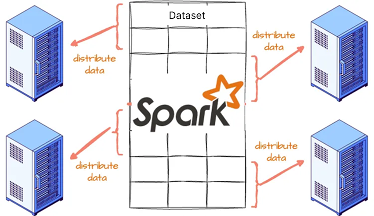
Figure A. Conceptual diagram of Apache Spark distributing large data chunks across physical machines (An original image edited by Kuriko IWAI)

Developed at UC Berkeley’s AMPLab in 2009 and later donated to the Apache Software Foundation, Spark distributes data and computations across multiple physical machines, allowing for parallel processing.

◼ Apache Spark Ecosystem

Apache Spark ecosystem has 3 main layers:

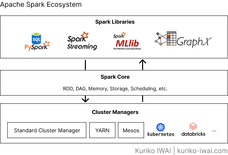
Figure B. The three-layer architecture of the Apache Spark Unified Ecosystem (Libraries, Core, Cluster Manager) (Created by Kuriko IWAI)

Spark Libraries (also known as the Spark Unified Libraries) (top, Figure B) consist of 4 high-level components built on top of a common engine:

• Spark SQL & DataFrames: Structured query processing, schema management, and relational data operations powered by the Catalyst Optimizer and Tungsten execution engine.

• Spark Streaming / Structured Streaming: Real-time stream processing that unifies batch and micro-batch/continuous processing with end-to-end exactly-once semantics.

• MLlib (Machine Learning Library): Scalable machine learning algorithms, feature engineering tools, and standardized Pipeline abstractions for model training and evaluation.

• GraphX: A distributed graph processing engine and API for graph-parallel computation and network analysis.

These high-level libraries call Spark Core (middle, Figure B) to translate code into data transformation and execute plans.

Then Spark Core requests and manages resources through the Cluster Manager (bottom, Figure B), schedule and execute tasks across worker nodes.

I'll walk you through this mechanism and process in the next section.

Spark operates using a master-worker architecture controlled by a driver program and executed across multiple worker nodes.

The below diagram shows the high level runtime architecture of Apache Spark:

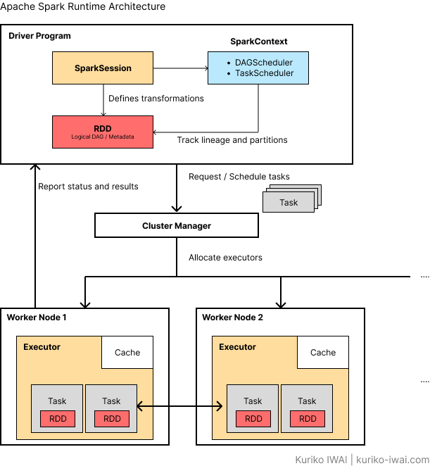
Figure C. High-level runtime architecture of Apache Spark showing driver, cluster manager, and executors (Created by Kuriko IWAI)

As Figure C shows, there are 5 primary components:

• Driver program (master node) (top, Figure C),

• Cluster manager (master node/orchestrator) (middle, Figure C),

• Worker node (bottom, Figure C),

• Executor, and

• Task.

◼ Driver Program

Driver program (or called driver) is the central coordinator node of a Spark application.

It translates code into DAG, tasks, and coordinates execution;

• Instantiates the SparkSession with its underlying SparkContext.

• Analyzes data transformations and actions.

• Breaks the execution into stages and tasks (each of which will be handled by an executor).

• Schedules tasks and sends them to individual executors.

• Collects final results.

◼ Cluster Manager

Cluster manager is the external service responsible for acquiring and allocating CPU/RAM resources across the worker nodes in the cluster.

It oversees the cluster of machines running the Spark application.

Spark can work with various cluster managers:

• Standalone: Spark's built-in, simple cluster manager.

• YARN: Hadoop's resource manager (common in traditional enterprise setups).

• Kubernetes (k8s): Container-based resource orchestration.

• Databricks Managed Cluster Manager: Auto-scaling cluster management native to Databricks.

◼ Worker Nodes

Worker nodes are the physical or virtual machines in the cluster that host executor processes.

They provide CPU, memory, and storage resources to run workloads.

They do not execute business logic directly; instead, they launch and manage executor processes.

◼ Executors

An executor is a dedicated distributed Java Virtual Machine (JVM) process launched on a worker node for a specific Spark application.

As Figure C shows, executors execute tasks the driver assigns and report their status and results:

• Runs individual Tasks assigned by the Driver across multiple CPU threads.

• Stores cached DataFrames/RDD partitions in memory (RAM) or disk.

• Persists until the application finishes or is dynamically terminated.

Each Spark application has its own set of executors, and a single worker node can host multiple executors.

◼ Tasks

A task is the smallest individual unit of work in Spark.

A single task represents the execution of a set of transformations on a single partition of data.

Figure C shows at least 4 tasks are created in 4 separate partitions, as an Resilient Distributed Dataset (RDD) has 4 partitions.

When an RDD (or DataFrame) has 100 partitions, Spark creates 100 tasks to process that stage.

Next section explains how RDD works.

Resilient Distributed Dataset (RDD) is the fundamental, low-level data abstraction in Apache Spark.

The below diagram shows how RDDs handle its core operations:

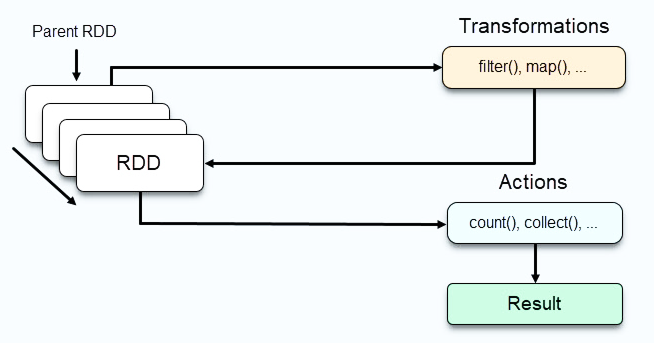
Figure D-1. RDD abstraction and core operations (Lazy transformations vs eager actions)

RDD is an immutable, read-only collection of data partitioned and distributed across worker nodes of a cluster.

RDD holds any type of data like Scala, Java, or Python objects (e.g., integers, strings, custom classes, or key-value tuples) in memory for as long and as much as possible.

◼ Core Operations - Transformations and Actions

As Figure D-1 shows, operations on an RDD fall into 2 categories:

• Transformations (lazy), and

• Actions (eager).

Transformations (and Lazy Evaluation)

Transformations are operations that create a new RDD from an existing one.

Examples include:

• .map()

• .filter()

• .groupByKey()

• .select()

• .filter()

• .join()

Transformations are lazily evaluated; Spark records the operation in a DAG, but does not execute it immediately.

Actions

Actions are operations that compute a result and return it to the Driver Program or write it to storage.

Examples include:

• .collect()

• .count()

• .saveAsTextFile())

Calling an action triggers actual computation across the cluster.

▫ Operational Flow

When we define the RDD, its inside data is not transformed immediately until an action triggers the execution.

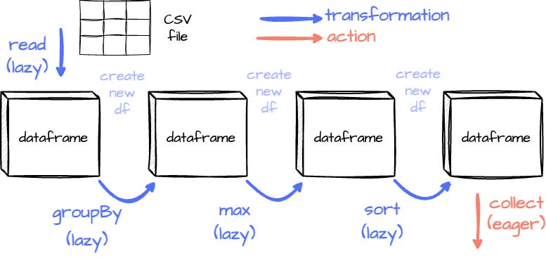
Figure D-2. Operational execution flow of RDD transformations, DAG building, and lineage graph evaluation

Figure D-2 shows that transformations first build a DAG plan, and when an action is called, the data is finally processed.

This approach allows Spark to determine the most efficient way to execute the transformations.

◼ Fault Tolerance

RDDs achieve fault tolerance through lineage.

As Figure D-2 shows, Spark forms the dependency lineage graph by keeping track of each RDD’s dependencies on other RDDs, which is the series of transformations that created the RDD.

When a worker node crashes and data in memory is lost, Spark simply uses this graph to recompute only the crashed node, completely skipping restarting the entire application.

◼ Benefits of Immutability

We know that RDDs are immutable; once created, it cannot be modified.

This means that any operation on an RDD produces a brand-new RDD rather than altering the existing one ("create new df" in Figure D-2).

This helps Spark in 3 ways:

• Concurrent processing: Immutability keeps data consistent across multiple nodes and threads, avoiding complex synchronization and race conditions. Spark can call multiple CPU cores to compute data simultaneously.

• Fault tolerance: Each transformation creates a new RDD, preserving the lineage and allowing Spark to recompute lost data reliably.

• Functional programming: RDDs follow functional programming principles that emphasize immutability, making it easier to handle failures and maintain data integrity.

◼ Anatomy of an RDD - The 5 Internal Properties

Every RDD in Spark is defined by 5 core properties:

1. List of partitions: Defines parallelism (How many tasks will run).

2. Computation function: Defines logic (How to iterate over and transform data).

3. Dependencies: Defines lineage & fault tolerance (How to reconstruct lost partitions).

4. Partitioner (optional): Defines data distribution (For key-value RDDs, how key-value keys are grouped across nodes).

5. Preferred locations (optional): Defines task placement (Where to run tasks to minimize network I/O).

◼ Partitions

Partitions is the array of discrete subsets into which the dataset is logically divided.

Spark cannot process a multi-terabyte file as a single monolith, so it splits the data into atomic units called partitions.

When an RDD is created, Spark divides the data into multiple chunks, known as partitions. Each partition is a logical data subset and can be processed independently with different executors. This enables Spark to perform operations on large datasets in parallel.

When a stage runs, Spark assigns one task per partition.

If an RDD has 100 partitions, Spark will launch 100 tasks to process them, running as many concurrently as there are available CPU cores/executor slots.

1from pyspark.sql import SparkSession
2
3# define spark session and context
4spark = SparkSession.builder.appName("app").getOrCreate()
5sc = spark.sparkContext
6
7# create an rdd with 4 explicit partitions
8rdd = sc.parallelize(range(1, 1000), numSlices=4)
9

For example, reading a 1 GB file with a 128 MB block size produces an RDD with 8 partitions.

◼ Computation Function

Computation function is an internal function that defines how to calculate the data for a given partition from its parent data.

Because RDDs are evaluated lazily, Spark doesn't immediately hold all data in memory; instead, it holds the recipe for computing it.

In the below code snippet, when the compute function is built, no worker node runs computation. Only when .collect() is called, the computation is triggered:

1from pyspark.sql import SparkSession
2
3# define spark session and context, create an rdd
4spark = SparkSession.builder.appName("app").getOrCreate()
5sc = spark.sparkContext
6rdd = sc.parallelize(range(1, 1000), numSlices=4)
7
8# build the compute function (even numbers x 10)
9filtered_rdd = rdd.filter(lambda x: x % 2 == 0)
10mapped_rdd = filtered_rdd.map(lambda x: x * 10)
11
12# calling .collect triggers the compute() method on each partition
13result = mapped_rdd.collect()
14

◼ Dependencies (Lineage)

Dependencies (or lineage) is a list of parent RDDs that the current RDD depends on, along with the nature of that dependency.

RDDs track their history to provide fault tolerance and build the DAG.

Spark classifies dependencies into two types:

• Narrow dependency (or called narrow transformation): Each partition of the parent RDD is used by at most one partition of the child RDD (e.g., map(), filter()). Data stays local on the node; no network shuffle is needed.

• Wide dependency (or called wide transformation): Multiple child partitions depend on data from a single parent partition (e.g., groupByKey(), join()). This triggers a shuffle, moving data across the network.

• Transformations: Narrow vs. Wide:

  Narrow Transformations: Each input partition contributes to exactly one output partition (e.g., map, filter). No network shuffle is required.

  Wide Transformations: Data across multiple partitions must be re-grouped across nodes (e.g., groupByKey, reduceByKey, join). This causes a Shuffle, which requires expensive network I/O and disk spillage.

If Worker Node B crashes and loses Partition #3, Spark uses the lineage to re-run only the compute() function for Partition #3 from its parent dependencies, rather than recomputing the entire dataset.

1from pyspark.sql import SparkSession
2
3# define spark session and context
4spark = SparkSession.builder.appName("app").getOrCreate()
5sc = spark.sparkContext
6
7# parent rdd
8rdd1 = sc.parallelize([("USA", 1), ("Canada", 2), ("USA", 3)])
9
10# narrow dependency: map() doesn't move data across network nodes
11rdd2 = rdd1.map(lambda x: (x[0], x[1] * 100))
12
13# wide Dependency: reduceByKey() requires a shuffle across the network
14rdd3 = rdd2.reduceByKey(lambda a, b: a + b)
15
16
17# inspect dependencies
18dependencies = rdd3._jrdd.dependencies()
19dependency_type = dependencies[0].getClass().getSimpleName()
20# dependncy_type returns ShuffleDependency
21

◼ Partitioner

A partitioner is an object that controls how key-value pair elements (RDD[(K, V)]) are routed to specific partition IDs.

For plain RDDs (e.g., text lines), the partitioner is None.

For key-value RDDs subjected to shuffle operations (like .reduceByKey() or .join()), Spark uses a partitioner:

• HashPartitioner: Calculates hash(key) % numPartitions to send rows with identical keys to the exact same partition/node.

• RangePartitioner: Sorts keys into ordered range buckets across partitions (used in .sortByKey()).

When two datasets are joined and already share the same partitioner, Spark skips the costly network shuffle during the join.

1from pyspark.sql import SparkSession
2
3# define spark session and context
4spark = SparkSession.builder.appName("app").getOrCreate()
5sc = spark.sparkContext
6
7# mock data
8data = [("A", "Emp1"), ("B", "Emp2"), ("A", "Emp3")]
9
10# plane rdd
11raw_rdd = sc.parallelize(data)
12raw_rdd.partitioner 
13# -> returns None
14
15
16# custom partition function to map key to rdd
17def custom_partition_func(key: str) -> int:
18    return 0 if key == "A" else 1
19
20# apply an explicit partitioner
21partitioned_rdd = raw_rdd.partitionBy(
22    numPartitions=2, 
23    partitionFunc=custom_partition_func,
24)
25partitioned_rdd.partitioner
26# -> returns `` 
27# confirming a partitioner object is actively attached to the rdd.
28

◼ Preferred Locations

Preferred locations are metadata specifying the physical IP addresses/hostnames where a given partition's source data resides.

Spark enforces the principle of data locality, indicating that moving computation to the data is cheaper than moving data to the computation.

When reading from storage systems like HDFS or Delta/S3, Hadoop Distributed File System (HDFS) tells Spark:

Spark’s scheduler reads preferredLocations() for Partition 1, sees Node-101, and attempts to assign Task 1 to an executor running on Node-101.

Locality levels: Spark attempts assignments in order of priority:

1. PROCESS_LOCAL (Data is already cached in the executor JVM).

2. NODE_LOCAL (Data is on the same physical server disk/HDFS block).

3. RACK_LOCAL (Data is on the same rack).

4. ANY (Data must be transferred over the network from another node).

1from pyspark.sql import SparkSession
2
3# define spark session and context
4spark = SparkSession.builder.appName("app").getOrCreate()
5sc = spark.sparkContext
6
7# read data from a distributed/locality-aware file system (e.g., HDFS/S3)
8file_rdd = sc.textFile("hdfs://namenode:9000/data/mock.csv")
9
10# get the jave rdd instance
11java_rdd = file_rdd._jrdd
12
13# query preferred locations for Partition 0
14first_partition = java_rdd.partitions()[0]
15preferred_hosts = java_rdd.preferredLocations(first_partition)
16
17# preferred_hosts: ['datanode101.internal', ...]
18

This section explains a complete, step-by-step breakdown of the Spark Execution Lifecycle, tracing the exact sequence of events from when we submit code to when results are returned.

◼ Step 1. Initializing the Driver

First, we submit a Spark application (via spark-submit, a Databricks Notebook cell, or an IDE).

The driver program process starts up, either locally or on a designated cluster node based on your deployment mode (I'll later explain).

Then, the driver creates a SparkSession and underlying SparkContext, which contacts the Cluster Manager to request compute resources.

1from pyspark.sql import SparkSession
2
3# driver process initializes to create a SparkSession
4spark = SparkSession.builder \
5    .appName("app") \
6    .master("local[*]") \
7    .config("spark.executor.memory", "2g") \
8    .getOrCreate()
9
10# create a SparkContext  
11sc = spark.sparkContext
12
13# the driver immediately transitions to step 2. executor allocation by requesting cpu cores and ram from the cluster manager.
14

◼ Step 2. Executor Provisioning & Registration

The cluster manager launches executor processes inside separate JVMs across the designated worker nodes.

Each executor registers back with the driver’s TaskScheduler, reporting its available CPU core slots and RAM capacity.

The cluster is now active, and the Driver is ready to parse your application code.

◼ Step 3. Building DAG

Spark reads each transformation then builds a node in a DAG, which tracks the lineage graph.

1# mock data
2mock_data = [("US", 10), ("CA", 20), ("US", 30), ("UK", 15)]
3
4# create a base rdd
5base_rdd = sc.parallelize(mock_data, numSlices=2)
6
7# create lineage graph
8filtered_rdd = base_rdd.filter(lambda x: x[1] > 12)
9mapped_rdd = filtered_rdd.map(lambda x: (x[0], x[1] * 2))
10

◼ Step 4. Catalyst Optimization

For DataFrame and SQL operations, the catalyst optimizer builds and optimizes the physical execution plan.

1# define a DataFrame pipeline
2df = spark.createDataFrame([
3    ("Alice", "Engineering", 90000),
4    ("Bob", "Engineering", 120000),
5    ("Charlie", "Sales", 80000)
6], ["name", "department", "salary"])
7
8# transformations build the catalyst logical plan
9processed_df = df \
10    .filter(df.salary > 85000) \
11    .select("name", "department")
12
13# inspect the complete catalyst planning pipeline
14processed_df.explain(extended=True)
15# output shows:
16# 1. Parsed Logical Plan
17# 2. Analyzed Logical Plan
18# 3. Optimized Logical Plan (Filter pushdown / column pruning)
19# 4. Physical Plan (WholeStageCodegen execution strategy)
20

◼ Step 5. Creating Stages

An action is called to trigger the DAGScheduler on the driver.

The DAGScheduler evaluates the logical DAG and breaks it into physical stages.

Then, the DAGScheduler passes each stage to the TaskScheduler.

◼ Step 6. Creating Tasks

The TaskScheduler splits each stage into individual tasks.

Each Task corresponds 1:1 with a single data partition.

The TaskScheduler then evaluates data locality via preferredLocations to figure out which executor holds or is closest to the physical data partition.

The driver dispatches these tasks to the available executor slots across the network.

1# wide transformation (reduceByKey) creates a shuffle boundary
2grouped_rdd = mapped_rdd.reduceByKey(lambda a, b: a + b)
3
4# calling an action (.collect()) triggers DAGScheduler & TaskScheduler execution
5result = grouped_rdd.collect()
6

◼ Step 7. Executing Tasks in Parallel

Executors receive the serialized task code from the driver, and run the tasks in parallel across their available CPU threads.

If a task requires caching (via .cache()), the partition results are saved in the executor’s memory storage space.

◼ Step 8. Shuffle for Multi-stage Execution

If the job has multiple stages, executors exchange data over the network during the shuffle phase.

Stage 1 tasks finish writing their output partitions into shuffle files on local executor disks.

Then, Stage 2 tasks wake up and pull their corresponding key-partitioned data over the network from Stage 1 executors.

Stage 2 tasks execute their logic once all required shuffle data is fetched.

1# inspect how data partitions were evaluated during execution across tasks
2def inspect_executor_task(partition_index, iterator):
3    data = list(iterator)
4    yield f"task on partition {partition_index} processed {len(data)} items: {data}"
5
6# collect partition execution layout from executors
7task_logs = grouped_rdd \
8    .mapPartitionsWithIndex(inspect_executor_task) \
9    .collect()
10

◼ Step 9. Results

Final output tasks complete and send their results back.

If saving to storage, executors directly write output files to the target file system/Data Lake in parallel.

If returning to the driver, executors serialize their output partition results back to the driver memory space.

1# write final DataFrame to persistent storage (distributed write across executors)
2df.write.mode("overwrite").parquet("/tmp/output_data.parquet")
3

◼ Step 10: Shutting Down the Application

The job reaches completion or the script finishes.

The SparkSession is closed via .stop() or notebook termination.

The driver notifies the cluster manager to release all allocated executor JVM processes and free CPU/RAM resources across the worker nodes.

1# stop SparkSession to shut down Executors and release driver resources
2spark.stop()
3

Spark offers different execution modes:

• Cluster mode,

• Client mode, and

• Local mode

which can run the execution lifecycle in its own way.

Below diagram shows the high-level concept, where the execution mode control where the driver runs, then the driver runs Spark lifecycle:

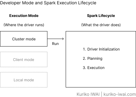
Figure E. Conceptual overview of Spark Application execution modes and its lifecycle (Created by Kuriko IWAI)

◼ Cluster Mode

Cluster mode is the production standard mode where the driver process is launched on a worker node within the cluster alongside the executor processes:

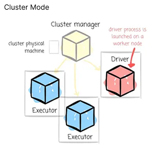
Figure F-1. Spark cluster mode execution architecture (Driver running inside the worker node)

In cluster mode, the client submits the job and disconnects; then the cluster manager handles all the processes related to the Spark application:

▫ Best Used For:

Automated production pipelines and scheduled batch jobs (e.g., airflow jobs) where network latency between driver and executors must be minimized.

◼ Client Mode

Client mode is the mode where the driver remains on the client machine that submitted the application:

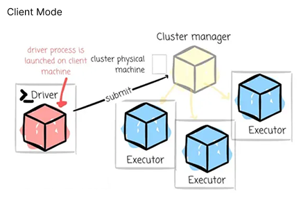
Figure F-2. Spark client mode execution architecture (Driver running on submitter edge machine).

In client mode, the driver process runs on the submitter's machine (e.g., laptop, an edge node, or a Databricks Notebook driver node), outside the worker cluster pool.

This setup requires the client machine to maintain the driver process throughout the application’s execution.

▫ Best Used For:

Interactive querying, data exploration, and REPL/Notebook development (e.g., Databricks interactive notebooks, Jupyter) where instant feedback is required.

◼ Local Mode

Local mode is the mode where the entire Spark application is ran on a single machine, achieving parallelism through multiple threads.

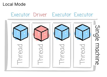
Figure F-3. Spark local mode architecture (Driver and executors co-existing in a single JVM process)

In local mode, there is no real cluster or cluster manager.

The driver and executor run inside the exact same JVM process on a single machine.

▫ Best Used For:

Unit testing, debugging PySpark code locally, and small-scale development on your laptop without spinning up a cluster.

◼ Comparing Execution Modes

Below table compares each execution mode with use case:

Table 1. Architectural comparison of Apache Spark execution modes (Cluster vs. Client vs. Local) (Created by Kuriko IWAI)

Spark was built to address the severe latency and disk I/O bottlenecks of classical MapReduce architectures.

Rather than writing intermediate state back to persistent disk after every map and reduce phase, Spark performs in-memory computing using persistent fault-tolerant abstractions.

Its typical use cases involve:

• Large-scale ML feature engineering: Computing complex aggregations, window functions, and embeddings over billions of rows.

• Distributed ML model inference: Scoring massive batch datasets using distributed PySpark UDFs or Spark Predictor pipelines.

• Real-time feature stores: Streaming continuous features into online/offline storage using Structured Streaming.

• ETL & Data lakehouse ingestion: Cleaning, deduplicating, and converting raw JSON/CSV logs into optimized Delta Lake format.

◼ Common Pitfalls

Although Spark is beneficial to handle large datasets, there are some common pitfalls.

▫ High Memory Footprint

JVM garbage collection overhead, memory leaks in Python worker processes, or unoptimized caching can cause Driver/Executor OutOfMemory (OOM) failures.

▫ Handling Skewed Data

If a key distribution is uneven (e.g., null keys or dominant IDs), one executor processes 90% of the data while others sit idle, causing severe stragglers.

▫ Small File Problem

Generating thousands of small partition files degrades read throughput and metastore query planning.

▫ PySpark Serialization Overhead

Converting data between JVM execution layers and Python worker processes (Py4J / IPC) introduces performance overhead when using non-vectorized Python UDFs.

◼ When to Use Spark

Understanding when to use Spark—and when not to—is important given pros and cons of Spark.

▫ Use Spark When:

• Data size exceeds single-node capacity: Your data cannot fit into high-memory VMs (e.g., 256GB+ RAM).

• Workloads require distributed compute: Feature calculations require distributed joins across massive multi-table data models.

• SLA-critical streaming is required: Real-time processing with low-latency streaming pipelines.

▫ Avoid Spark When:

• Data fits easily in single-node RAM: Datasets under ~20–50 GB can be processed faster with single-node tools like Pandas, Polars, or DuckDB without cluster initialization and serialization overhead.

• Purely iterative single-node ML algorithms: Training standard, non-distributed Scikit-Learn models on small datasets.

Written by Kuriko Iwai · Kernel Labs. All images, unless otherwise noted, are by the author. All experimentations on this blog utilize synthetic or licensed data.

FAQ

Share What You Learned

Continue Your Learning

If you enjoyed this blog, these related entries will complete the picture:

Related Books for Further Understanding

These books cover the wide range of theories and practices; from fundamentals to PhD level.

Linear Algebra Done Right

Foundations of Machine Learning, second edition (Adaptive Computation and Machine Learning series)

Designing Data-Intensive Applications: The Big Ideas Behind Reliable, Scalable, and Maintainable Systems

Machine Learning Design Patterns: Solutions to Common Challenges in Data Preparation, Model Building, and MLOps