How to Solve Time-Varying Confounding & Mediator Bias in Longitudinal ML Pipelines

[Series] Causal Machine Learning - 3. De-Biasing Sequential Telemetry and Multi-Period Decisions

By Kuriko IWAI

Table of Contents

Real-world enterprise environments are not single-step games.

Once an initial action is taken, the ecosystem doesn’t remain passive—downstream telemetry evolves dynamically, and mid-game course corrections break static causal assumptions.

This structural feedback loop creates the time-varying trap, where intermediate system metrics act simultaneously as mediators of past actions and confounders of future decisions.

Standard machine learning (ML) models severely break under these conditions, triggering mediator-blocking bias and collider stratification bias.

In this article, I break down the mathematics of sequential exchangeability and demonstrate how Marginal Structural Models (MSMs) utilize time-varying Inverse Probability of Treatment Weighting (IPTW) to calculate unconfounded total causal effects with Python code.

Time-varying trap (or time-varying confounding) indicates a complex scenario in sequential, multi-period data where a variable measured over time acts simultaneously as a mediator and a confounder.

Below diagram shows how system states evolve over a multi-period horizon:

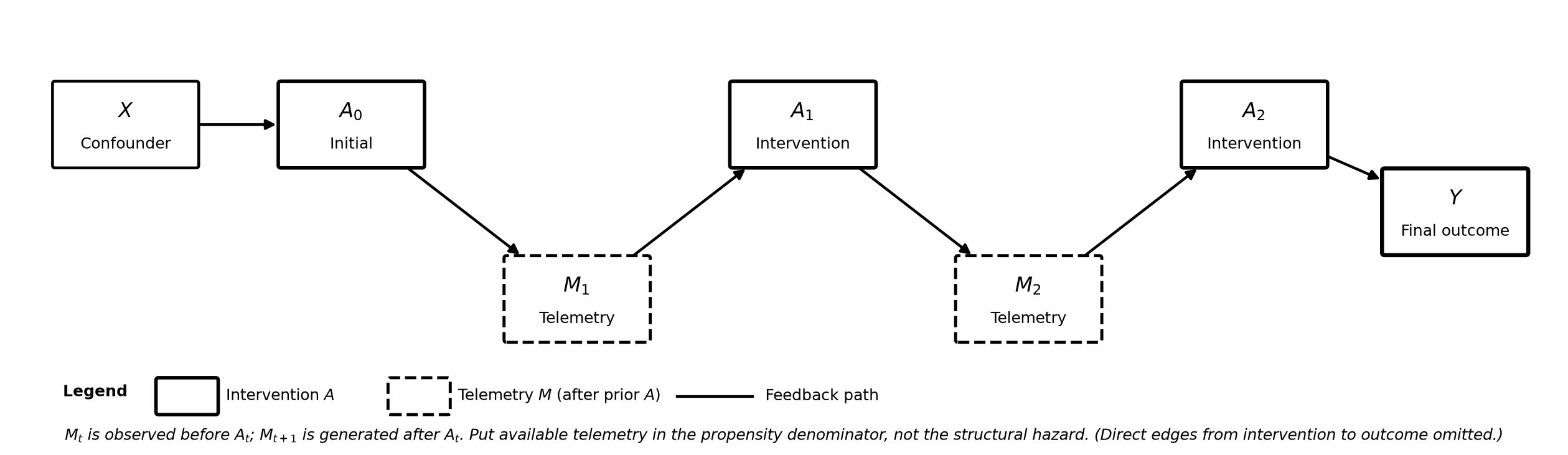
Figure A. Longitudinal Directed Acyclic Graph (DAG) showing time-varying confounding and telemetry dual-roles in enterprise employee retention (Created by Kuriko IWAI)

Let us consider an enterprise employee retention pipeline across two time steps.

The figure include key components:

• Confounder X: The employee's background and professional experience.

• Initial intervention A_0: Day1 onboarding program assignment.

• Month-1 telemetry M_1: Engagement of the employee (M_1 = 1 indicates high engagement).

• Month-1 intervention A_1: Manager's check-ins in Month 1.

• Final outcome Y: Retention of the employee at the end of temporal horizon (i.e., T = 12 months).

◼ The Dual-Role of Telemetry - Mediator AND Confounder

Here, M_1 is a mediator because the initial intervention improves it.

For instance, if an employee had good onboarding experience, they'd be likely to engage more (A_0 = 1 → M_1 = 1).

But M_1 is also a confounder because a sudden drop in engagement could trigger A_1 (manager's check-ins) and directly lower retention Y.

M_1 is directly impacted by the past interventions, but also impacts on future interventions, and hence, the final outcome.

Because M_1 plays both roles over time, static feature-flattening models fail to isolate the true causal effect of this continuous sequences.

In static ML, we only worry about baseline confounder X.

But in sequential systems we saw in the previous section, past interventions pollute future states.

This makes static ML face a structural dilemma.

◼ The True Causal Effect

Imagine we have 1,000 software engineers in our staffing pipeline.

When we split them into two groups:

1. Group 1. (500 engineers) Receives intensive onboarding (A_0 = 1), and

2. Group 2. (500 engineers) Receives standard onboarding (A_0 = 0).

Below diagram demonstrates how the true causal effect is measured for retention at temporal horizon T:

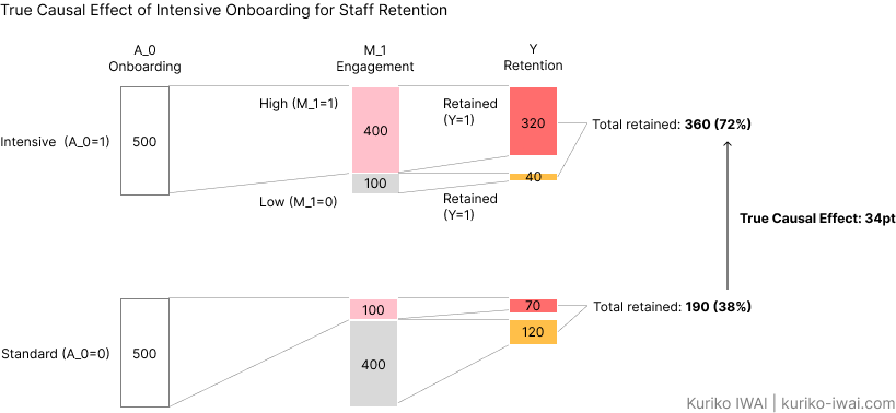
Figure B-1. True total causal effect of multi-period interventions on long-term retention (Created by Kuriko IWAI)

Among 500 engineers under the intensive onboarding (upper row, Figure B-1), 400 engineers had high engagement at Month 1, and 320 engineers were retained.

The remaining 100 developers had low engagement, but 40 engineers were retained.

So, in total, the intensive onboarding achieved 72% of retention rate; compared to 38% of standard onboarding (bottom row, Figure B-1), boosting the retention rate by 34 points.

◼ Mediator-blocking Bias

Native ML models control for M_1 by including M_1 in the feature set.

However, this accidentally blocks the indirect causal path of the initial intervention A_0:

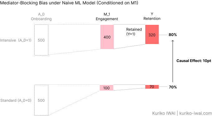
Figure B-2. Mediator-blocking bias misestimates causal effect due to covariate over-adjustment (Created by Kuriko IWAI).

Figure B-2 demonstrates mediator-blocking bias (or over-adjustment bias) where when an ML model conditioned on M_1, it completely misses the benefit of intensive onboarding (A_0 = 1) which drives 80% of developers into high engagement (M_1 = 1), instead of just 20%.

▫ Mathematical Background of Mediator-blocking Bias

Suppose our data science team attempts to evaluate the retention strategy by fitting a standard multi-variable regression model:

where β's represent weights assigned to each variable and k represents temporal horizon such as k=12.

Eq. 1 includes M_1 because we correctly identify that M_1 is a confounder for A_1.

This, however, blocks the indirect causal path from A_0 to Y, dampening weight β_0 which measures the Controlled Direct Effect (CDE) of A_0 on the final outcome.

On the other hand, the model attributes credit for M_1, even though A_0 actually caused M_1, assigning a large value to β_1.

Stakeholders looking at large β_1 might say: "Month 1 engagement (M_1) drives employee retention. Let's focus on engagement.", missing the fact that M_1 was a result of the onboarding program (A_0).

Table 1. Ground Truth vs. Naive ML Conditioning on Time-Varying Mediators (Created by Kuriko IWAI)

◼ Selection Bias

When we exclude M_1 from the feature set, the estimation of the secondary intervention A_1 suffers from uncontrolled baseline confounding.

Selection bias occurs in two situations:

1. Confounder selection bias: Failing to control for baseline X when assigning onboarding, so the model analyzes non-randomly selected samples.

2. Collider stratification bias: Conditioning on a variable that creates a fake correlation between two independent variables; for example, evaluating manager interventions (A_1) by filtering the dataset strictly to low-engagement developers (M_1 = 0).

◼ Confounder Selection Bias

Suppose Senior Engineers (X = 1) inherently retain at higher rates (80%), but managers preferentially send Junior Engineers (X = 0) to the intensive onboarding program (A_0 = 1) because they need more help:

• Senior Engineers (X = 1, 500 total): Naturally retained at 80%. Only 100 were assigned to the intensive program.

• Junior Engineers (X = 0, 500 total): Naturally retained at 40%. 400 were assigned to the intensive program.

Below diagram demonstrates confounder selection bias:

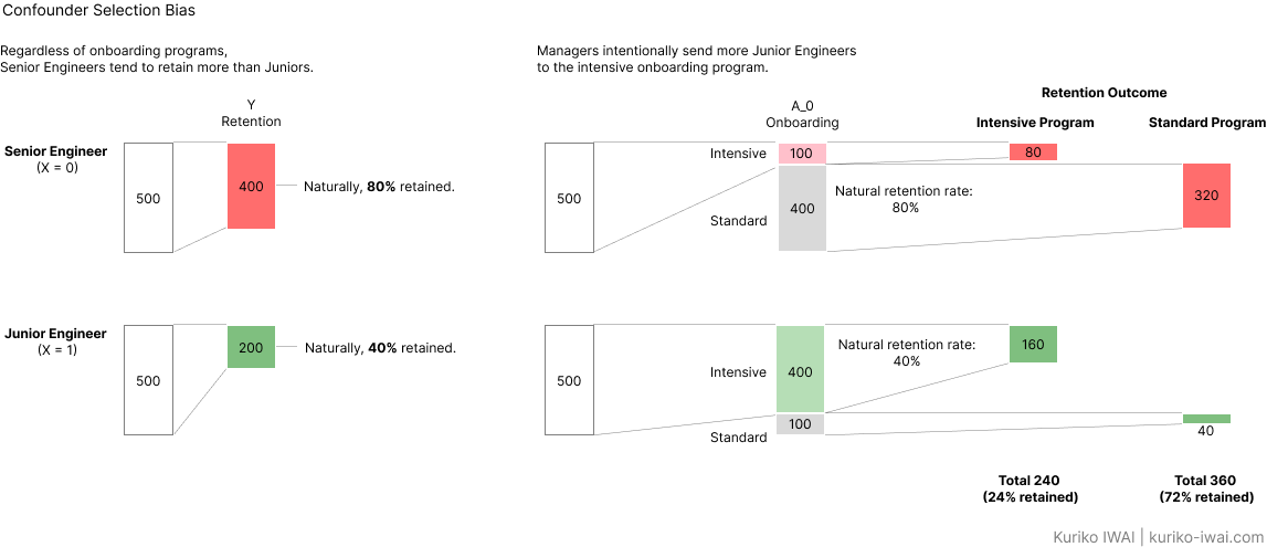
Figure C-1. Confounder selection bias resulting from non-random treatment assignment across baseline demographics (Created by Kuriko IWAI)

When the analyst simply compares retention rates after the intensive and standard onboarding program, standard has much higher rate (72%, right, Figure C-1) than intensive (24%, middle, Figure C-1).

But the truth is that the sample receiving the intensive program was heavily biased toward Junior Engineers who naturally leave at higher rates.

Here, intensive onboarding wasn't failing at all—it was handed a fundamentally harder population: Junior Engineers.

◼ Collider Stratification Bias

Collider stratification bias is a subtle form of selection bias where conditioning on a middle variable (M_1) artificially creates an inverted correlation between two unlinked factors.

Suppose two unlinked factors cause low engagement (M_1 = 0):

1. Standard onboarding (A_0 = 0), and

2. Personal burnout / external hardship (U = 1).

Suppose leadership asks:

By restricting the analysis strictly to low-engaging engineers (M_1 = 0), the model confuses that the intensive onboarding causes low engagement.

But in reality, these engineers had low engagement not because of poor onboarding, but because of personal burnout (U = 1, left, Figure C-2).

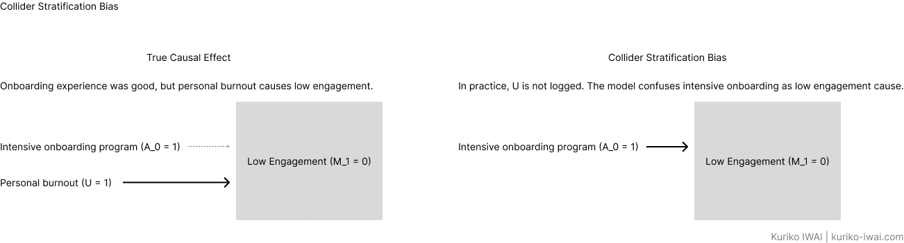
Figure C-2. Collider stratification bias induced by conditioning on intermediate telemetry affected by unobserved confounders (Created by Kuriko IWAI).

Here, M_1 is a collider because two separate factors (A_0 and U) point directly into it.

And U represents factors like personal family emergencies, mental fatigue, bad team dynamics, or sudden external hardships.

In real-world enterprise telemetry, U is rarely logged or quantifiable.

Because U remains unobserved and hence, omitted from the regression model, filtering on M_1 = 0 forces A_0 to act as a proxy of U.

So, how can we know if we have recorded enough history to calculate true cause-and-effect?

Sequential exchangeability tackles these challenges by structurally completing the causal pipeline, extending Judea Pearl's backdoor criterion across time t:

where \bar{H}_t represents historical trajectory up to time step t:

where \bar{A}_{t-1} and \bar{M}_t represent a complete sequence of past interventions up to step t-1 and post-treatment intermediate states up to step t, respectively.

In this concept, the decision to assign intervention A_t is independent of the potential counterfactual outcome Y(\bar{a}), indicating that there's no unobserved confounders affecting intervention A_t at any stage of the pipeline, once historical trajectory is defined.

◼ How Sequential Exchangeability Solves Both Biases

Sequential exchangeability is the theoretical backbone that powers Inverse Probability of Treatment Weighting (IPTW) and Marginal Structural Models (MSMs).

▫ Eliminating Selection Bias

First, it eliminates selection bias at every step.

IPTW calculates time-varying weights:

These weights construct a synthetic pseudo-population where intervention A_t is pseudo-randomized relative to past history.

This can strip away the selection bias because A_t is no longer determined by past history \bar{H}_t, breaking the confounding links that caused the bias in the first place.

▫ Eliminating Mediator-blocking bias

Instead of putting M_1 directly into the regression model, sequential exchangeability uses M_1 only to construct the propensity weights W_t.

For a two-stage longitudinal pipeline with initial intervention A_0, intermediate state M_1, and secondary treatment A_1, the cumulative unstabilized weight W is the product of the inverse propensity scores at each time step:

where:

• Weight at time t=0 (W_0) for individual i inversely models the probability of receiving initial intervention A_0 given baseline confounder X, and

• Weight at time t=1 (W_1) for individual i inversely models the probability of receiving secondary treatment A_1 given the full prior trajectory \bar{H}_1 = {X, A_0, M_1}.

This unstabilized weight can produce extreme values (large variance) if some intervention probabilities are very small.

In practice, we use Stabilized Weights (SW), which replace the numerator 1 in Eq. 3.2 with the probability of the current intervention conditioned only on past intervention history:

where A_0 and A_1 represent interventions at t = 0 and t = 1 respectively.

Eq 3.3.1 can be generalized with T time steps:

Once SW_i (Eq. 3.3.2) is calculated for every individual, we can fit a weighted regression model for final outcome Y using only the intervention history variables (A_0, A_1), completely excluding M_1:

Because M_1 was used to construct SW_i (included in the past history), the sample is reweighted to break the confounding links, while leaving the mediator path (A_0 -> M_1 -> Y) open.

Now, β_1 successfully captures the true total causal effect (+34pt) of the intensive onboarding program.

Also, the model does not stratify on post-treatment status, preventing A_0 from becoming a proxy for unobserved factors (U).

This section demonstrates how an outcome changes when evaluating a continuous policy sequence versus evaluating single-step isolated decisions.

◼ Model Selection

I'll select a following models:

1. Standard Regression

• Serves as the baseline benchmark to demonstrate traditional model failure modes.

• Shows what happens when we either ignore confounders (inducing baseline selection bias) or include intermediate variables directly in the feature space.

2. Static IPS

• Corrects for single-point baseline confounding at time t=0 (X -> A_0).

• Re-weights the population so intervention and control groups look balanced at baseline.

3. Long Short-Term Memory (LSTM)

• Acts as a flexible, non-linear propensity estimator for complex, high-dimensional longitudinal histories.

• Captures non-linear dependencies, sequential patterns, and long-term history across time steps without requiring manual feature engineering of historical trajectories.

4. MSM

• Represents the gold-standard causal model for longitudinal data with time-varying confounding and mediation.

• Uses intermediate variables strictly to build sequential IPTW weights while leaving M_1 out of the final outcome regression.

◼ Interventional Policy Evaluation in Action

Now, let us compare the four models.

First, I'll define the synthetic data:

1import torch
2import numpy as np
3import pandas as pd
4
5# set seed for reproducibility
6np.random.seed(42)
7torch.manual_seed(42)
8
9N = 2000
10
11# X: experience level (1: senior, 0: junior)
12X = np.random.binomial(1, 0.5, N)
13
14# A_0: onboarding (Juniors targeted more heavily)
15p_A0 = 1 / (1 + np.exp(-(-0.8 * X + 0.2)))
16A0 = np.random.binomial(1, p_A0)
17
18# U: unobserved elements (personal burnout)
19U = np.random.binomial(1, 0.3, N)
20
21# M1: month-1 engagement driven by A_0 and U
22p_M1 = 1 / (1 + np.exp(-(1.2 * A0 - 2.0 * U + 0.5)))
23M1 = np.random.binomial(1, p_M1)
24
25# A1: secondary check-in (target heavly for low engagement M_1=0)
26p_A1 = 1 / (1 + np.exp(-(-1.5 * M1 + 0.5 * X)))
27A1 = np.random.binomial(1, p_A1)
28
29# Y: final retention outcome
30y_logit = -0.5 + 0.8 * A0 + 1.2 * M1 + 0.6 * A1 + 1.0 * X - 2.5 * U
31p_Y = 1 / (1 + np.exp(-y_logit))
32Y = np.random.binomial(1, p_Y)
33
34# create a pandas df
35df = pd.DataFrame({"X": X, "A0": A0, "M1": M1, "A1": A1, "Y": Y})
36

Next, I'll define and train the models:

1import numpy as np
2import pandas as pd
3import statsmodels.api as sm
4import statsmodels.formula.api as smf
5import torch
6import torch.nn as nn
7
8# 1. standard regression
9model_standard = smf.logit("Y ~ A0 + M1 + A1 + X", data=df).fit(disp=0)
10
11
12# 2. static IPS
13ps_model_a0 = smf.logit("A0 ~ X", data=df).fit(disp=0)
14df["ps_a0"] = ps_model_a0.predict(df)
15df["w_static"] = np.where(df["A0"] == 1, 1 / df["ps_a0"], 1 / (1 - df["ps_a0"]))
16
17# fit outcome model with static weights (excluding M1)
18model_static_ips = smf.wls(
19    "Y ~ A0 + A1", data=df, weights=df["w_static"]
20).fit()
21
22
23# 3. lmst
24class LongitudinalPropensityLSTM(nn.Module):
25
26    def __init__(self, input_dim, hidden_dim):
27        super().__init__()
28        self.lstm = nn.LSTM(input_dim, hidden_dim, batch_first=True)
29        self.fc = nn.Linear(hidden_dim, 1)
30
31    def forward(self, x):
32        lstm_out, _ = self.lstm(x)
33        # Output probability for treatment at each time step
34        probs = torch.sigmoid(self.fc(lstm_out))
35        return probs
36
37# format time steps: [t0_features (X), t1_features (X, A0, M1)]
38X_t0 = np.column_stack([df["X"], np.zeros(N), np.zeros(N)])
39X_t1 = np.column_stack([df["X"], df["A0"], df["M1"]])
40seq_data = torch.tensor(
41    np.stack([X_t0, X_t1], axis=1), dtype=torch.float32
42)  # shape: (N, 2, 3)
43
44lstm_model = LongitudinalPropensityLSTM(input_dim=3, hidden_dim=8)
45predicted_probs = lstm_model(seq_data).squeeze().detach().numpy()
46
47
48# 4. msm
49# numerators (P(A_t | A_{t-1}))
50num_a0 = smf.logit("A0 ~ 1", data=df).fit(disp=0).predict(df)
51num_a1 = smf.logit("A1 ~ A0", data=df).fit(disp=0).predict(df)
52
53p_num_a0 = np.where(df["A0"] == 1, num_a0, 1 - num_a0)
54p_num_a1 = np.where(df["A1"] == 1, num_a1, 1 - num_a1)
55
56# denominators (P(A_t | History_t))
57den_a0 = ps_model_a0.predict(df)
58den_a1 = smf.logit("A1 ~ A0 + M1 + X", data=df).fit(disp=0).predict(df)
59
60p_den_a0 = np.where(df["A0"] == 1, den_a0, 1 - den_a0)
61p_den_a1 = np.where(df["A1"] == 1, den_a1, 1 - den_a1)
62
63# cumulative stabilized weights
64df["sw"] = (p_num_a0 / p_den_a0) * (p_num_a1 / p_den_a1)
65
66# fit msm on pseudo-population
67msm = smf.wls("Y ~ A0 + A1", data=df, weights=df["sw"]).fit()
68Results
69

◼ Results

I estimated the initial onboarding and first manager check-in effects (β^​A_0​​ and β^​A_1​​), and measured biases from the ground truth.

The below table compares the results:

Table 2. Numerical Causal Model Validation and Bias Comparison Matrix (Created by Kuriko IWAI)

▫ Standard Regression

Standard regression suffers mediator blocking bias (-0.58) as well as collider stratification (-0.48).

Conditioning on M_1 in the feature space forces A_1 to act as a proxy on unobserved elements (U).

▫ Static IPS

Static IPS successfully re-weights A_0, making the bias near zero, but causes severe bias on A_1 (-0.42) because it omits M_1 from t = 1 propensity scores.

▫ LSTM

Without causal re-weighting, LSTM relies on conditional probability P(Y | A, H), underestimating early actions (-0.45). Then, it over-inflates the manager's check-ins (+0.28), confusing high managerial focus on risk profiles for treatment efficacy.

▫ MSM

MSM successfully recovers both ground truth targets.

MSM can re-weights the observational trajectory using sequential propensity scores.

It uses intermediate states (M_1) strictly to construct time-varying weights, then removes it from the final outcome model.

Here is the summary of key production health check metrics:

Table 3. Production Health Check and Operational Risk Matrix for Longitudinal Causal Models (Created by Kuriko IWAI)

Understanding dual-role variables and sequential exchangeability provides the structural framework for multi-period causal modeling.

But mathematical graph theory is useless if your underlying database telemetry is a chaotic mess.

In Part 4, we will step out of the math and into the data engineering trenches to build a timestamp architecture that enforces chronological ordering in production.

Written by Kuriko IWAI. All images, unless otherwise noted, are by the author. All experimentations on this blog utilize synthetic or licensed data.

FAQ

Share What You Learned

Continue Your Learning

If you enjoyed this blog, these related entries will complete the picture:

• Why Machine Learning Demands Causal Inference

  

  Eliminate selection bias and structural confounding. Learn do-operator, graph surgery, backdoor criterion.

• Fixing Selection Bias in Enterprise Data with Inverse Propensity Scoring (IPS)

  

  Fix selection bias in observational data with IPS. Learn propensity math, positivity limits, and Python implementation.

Related Books for Further Understanding

These books cover the wide range of theories and practices; from fundamentals to PhD level.

Linear Algebra Done Right

Foundations of Machine Learning, second edition (Adaptive Computation and Machine Learning series)

Designing Data-Intensive Applications: The Big Ideas Behind Reliable, Scalable, and Maintainable Systems

Machine Learning Design Patterns: Solutions to Common Challenges in Data Preparation, Model Building, and MLOps

Hands-On Large Language Models: Language Understanding and Generation