Apache Spark Internals Explained: RDDs, JVM, Jobs, Stages, Tasks & Shuffle

A practical deep dive into Spark distributed execution model, executor, shuffle mechanics, and DataFrame query optimization.

Kuriko Iwai · Kernel Labs

Machine Learning · fine-tuning · GraphRAG · causal ML

Table of Contents

As datasets grow, processing them efficiently on a single machine can become challenging due to limitations in CPU capacity, memory, and storage throughput.

Apache Spark addresses these challenges by providing a distributed data processing engine that can divide workloads into partitions and execute tasks in parallel across CPU cores and multiple machines.

However, Spark is not simply about adding more machines.

Understanding how its components work together—Drivers, Executors, RDDs, DataFrames, Partitions, Jobs, Stages, and Tasks—is essential to designing efficient and reliable data pipelines.

In this article, I'll walk through Spark's architecture, execution mechanics, and key performance considerations using a practical e-commerce sales aggregation example, with structured query planning and optimization.

Apache Spark is a distributed computing engine.

Below diagram shows parallel data processing on Spark, comparing a single node execution:

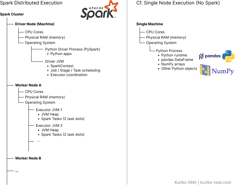
Figure A. High-level Apache Spark distributed cluster architecture (cluster, driver, and worker nodes), comparing a single node execution (Created by Kuriko IWAI)

As you can see on the left side, Spark divides work into tasks that can execute across CPU cores and, when available, across machines.

Spark is useful for large-scale ETL, SQL analytics, feature engineering, and many data processing workloads.

Distributed does not mean multiple machines are mandatory.

Spark can run in local mode on a single machine. Even there, data can be partitioned and processed in parallel.

◼ E-Commerce Use Case: Input Dataset Overview

Let us imagine a boutique e-commerce company.

It has 10,000 sales records, each with a stock keeping unit (SKU) and quantity sold.

Assume three possible SKUs: A, B, and C.

Table 1. E-Commerce sales record breakdown & expected aggregations (Created by Kuriko IWAI)

Our goal is to calculate total valid units sold per SKU:

1. Filter out records whose qty <= 0, then

2. Aggregate samples by SKU.

In the illustrative full dataset, suppose 9,800 of the 10,000 records remain after filtering and the final totals are:

1[("A", 8000), ("B", 10500), ("C", 9200)]
2

These totals are illustrative, not computed from the five-row sample above.

The Driver coordinates a Spark application. It maintains application state, constructs and schedules work, and communicates with executors. The Cluster Manager allocates resources under the deployment's resource-management system. Worker nodes supply compute resources. Executors are processes that execute tasks and hold data such as cached partitions and shuffle data.

It is important to distinguish these concepts: a worker is a machine or compute node; an executor is a process running on a node; and a task is a unit of work run by an executor. A worker can host multiple executors depending on cluster configuration. Some managed environments commonly use one executor per worker, but this is not a universal Spark rule.

◼ Simplified Cluster

First, we assume the following setups:

▫ Worker Nodes (Workers)

Worker Node (or Worker) is a machine to compute on Spark, like an instance to run the computational process.

I'll set 3 worker nodes, each of which has a spec (instance type) of 8 vCPU with 32 GiB RAM:

Figure B. Resource allocation across Worker Nodes (Created by Kuriko IWAI)

So, in total, 24 vCPU are available in the system.

▫ Spark Executors and CPU/Memory Allocation

Let's say, I'll secure:

• 7 Spark Executors (Executors) in total.

• 2 vCPU cores for each Executor.

• 3GiB JVM heap memory for each Executor.

Based on this setup, Spark Application requests Cluster Manager to allocate resources to the 7 Executors.

Then, Cluster Manager decides how to allocate CPUs and memory based on the resource usage of each Worker:

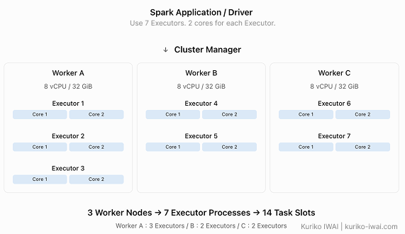
Figure C-1. vCPU cores, memory, and Executor allocation across Workers with resource imbalance in Worker A (Created by Kuriko IWAI)

Figure C-1 shows that the allocation creates 14 task slots (2 vCPU core x 7 Executors).

Note that the 3 GiB memory allocated to Executor is not its total memory because it has to secure memory overhead for Workers and other executions.

Under the assumption a single task requires 1 vCPU (spark.task.cpus = 1), each Worker allocates its vCPU:

Figure C-2. Parallel vCPU allocation across Workers (Created by Kuriko IWAI)

This shows two points:

1. Each Worker has its unique CPU usage rate (In Figure C-2, Worker A is 75%, while Workers B and C are 50%).

2. Even though the system has 24 vCPU cores (8 vCPU/Worker x 3 Workers), it can only use 14 vCPU cores; the rest 10 remain unused for these Tasks.

In some ecosystems like Databricks, 1 Worker has 1 Executor by default.

An RDD (Resilient Distributed Dataset) is an immutable, partitioned collection of elements that Spark can process in parallel. RDDs track dependencies between transformations, allowing Spark to recompute lost partitions in many failure scenarios.

The name captures three properties:

• Resilient: Spark records lineage—which RDD depends on which previous RDD—and can often reconstruct missing partitions instead of maintaining replicas of every intermediate result.

• Distributed: The dataset is represented as partitions that Spark may process on different executors. Multiple physical machines are not required; local mode also supports RDDs.

• Dataset: An RDD can contain key-value pairs, integers, strings, tuples, and other supported elements—not only relational rows. RDD APIs include operations such as map, filter, reduceByKey, join, and aggregateByKey.

An RDD is a logical collection and computation abstraction, not a declaration that particular partitions are permanently assigned to particular workers.

◼ Partitions

A partition is a logical chunk of data and normally corresponds to one task within a stage.

Let's say we create 100 partitions (These 100 initial partitions are an explicit teaching choice).

With 10,000 source elements, it gives approximately 100 elements per partition if the input is distributed roughly evenly:

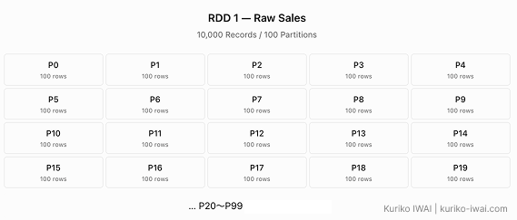
Figure D. Parallel partition allocation across 100 initial data splits (Created by Kuriko IWAI)

Note that equal distribution is not a general guarantee, particularly after filtering or shuffling.

To achieve the goal of computing the aggregate number of goods sold by SKU, we follow the seven steps:

Step 1. Create a SparkSession.

Step 2. Define raw sales RDD with 100 partitions.

Step 3. Define the filtered RDD.

Step 4. Define the SKU aggregation RDD with four output partitions.

Step 5. Trigger an action; Spark determines jobs, stages, and tasks.

Step 6. Executors execute tasks, subject to 14 available task slots.

Step 7. Return the small aggregated result to the Driver.

We use the RDD API in this walkthrough because it makes Spark's partitions, dependencies, shuffle boundaries, and task execution easier to observe.

For most modern structured data pipelines, the DataFrame API is generally the preferred starting point, as we will explore later.

◼ Step 1. Create a SparkSession

First, SparkApplication creates a SparkSession:

1from pyspark.sql import SparkSession
2
3# step 1 - create sparksession
4spark = SparkSession.builder.appName("app1").getOrCreate()
5sc = spark.sparkContext
6

As we saw in the previous section, this process includes ClusterManager to decide CPU/Memory allocation to each Worker:

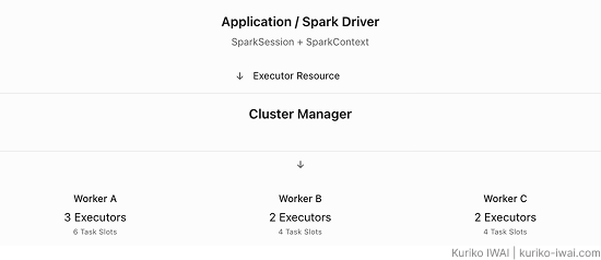
Figure E. Cluster manager to allocate tasks to Workers (Created by Kuriko IWAI)

Here, SparkSession is the normal entry point for DataFrame and SQL operations.

SparkContext is the entry point for the core RDD API. The exact creation and resource-allocation lifecycle depends on deployment mode and cluster configuration.

◼ Step 2. Define RDD 1: Raw Sales

Assume records is an existing Python collection of 10,000 (sku, qty) tuples; the complete contents are intentionally omitted from this note.

1raw_rdd = sc.parallelize(records, 100)
2

sc.parallelize() is convenient for small teaching examples, because the data begins in the Driver's Python process. It is usually not the preferred ingestion method for a huge production dataset. For large datasets, read from distributed storage with Spark readers instead.

Figure C shows that each Partition (P0, P1, ...P99) has 100 rows (samples) in total.

For instance, P0 (Partition 0) in RDD 1 looks like:

Table 2. Sample Raw Data Partition Layout (Partition 0 - Row Level View) (Created by Kuriko IWAI)

◼ Step 3. Define RDD 2: Filter Invalid Quantities

Next, RDD 2 has created to filter invalid records:

1filtered_rdd = raw_rdd.filter(lambda row: row[1] > 0)
2

filter is a narrow transformation: the output of an individual partition depends only on the corresponding input partition.

The number of partitions remains 100, although the number of records per partition may change.

Suppose this filter removes 200 invalid records. Then 9,800 remain, equivalent to 98 records per partition on average, not 98 in every partition:

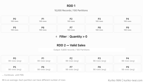
Figure F. From RDD 1 to RDD 2. Row filtering flow across 100 partitions (Created by Kuriko IWAI)

◼ Step 4. Define RDD 3: Aggregate Sales by SKU

The last RDD is to group the data by SKU, creating 4 output Partition:

1result_rdd = filtered_rdd.reduceByKey(
2    lambda a, b: a + b,
3    numPartitions=4 # human to define the num of output partitions
4)
5

This combines quantities with the same SKU key. reduceByKey performs map-side combining before shuffling partial results to the four reduce partitions.

Important: reduceByKey demonstrates why the statement “RDDs only support row-wise transformations” is incorrect. RDDs can perform aggregations and many other distributed operations.

So, after RDD2, RDD 3 would look like the following:

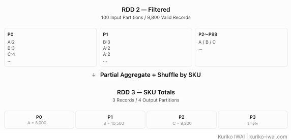
Figure G. From RDD 2 to RDD 3. Data redistribution during reduceByKey Aggregation across 4 reduce partitions (Created by Kuriko IWAI)

In practice, Hash Partitioner allocates SKUs to Partitions.

This hash-based partitioning strategy is common, but the actual distribution of the three SKUs over four reduced partitions depends on hashing and configuration. Some partitions may have zero resulting keys.

So, to summarize Steps 2 to 4:

Table 3. Summary of RDD lineage transformations and partition count evolution (Created by Kuriko IWAI)

◼ Lazy Evaluation and Lineage

The filter and reduceByKey calls establish a dependency graph; they do not immediately compute the full aggregation.

Spark records how to produce filtered_rdd from raw_rdd and result_rdd from filtered_rdd.

It is important to note that no Worker has been assigned to the RDDs yet, hence, no computation happens at this stage.

This is called lazy evaluation where Spark only defines how to transform data with RDDs, while postponing the execution of such transformation in a later phase.

The RDD lineage view looks like a graph of what depends on what:

raw_rdd: 100 partitions

→ filtered_rdd: 100 partitions

→ result_rdd: 4 partitions

→ Driver-side Python list

◼ Step 5. Trigger an Action

After defining RDDs, Driver decides Shuffle Boundary, where RDDs are divided into separate Stages, and schedules these Stages.

1result = result_rdd.collect()
2

collect() is an action. It starts computation required to produce the RDD and returns all output elements to the Driver.

Here only three SKU aggregates are expected, so collect() is reasonable. But collecting millions of records to a Driver can exhaust Driver memory.

Spark uses the RDD dependencies to build an execution plan, breaking the work into stages and tasks. For our simplified example, expect a shuffle map stage before the reduceByKey shuffle and a result stage after it.

◼ Jobs, Stages, Tasks—Their Relationship to RDD Lineage

A job refers to the scheduler work associated with computing an action's result.

A stage refers to a set of tasks separated from other stages by scheduling dependencies such as shuffle.

A task is work for one partition within a stage.

In our case, Driver decides to set Shuffle Boundary between RDDs 2 and 3, creating Stage 1 with RDDs 1 and 2, and Stage 2 with RDD 3 in Job 1:

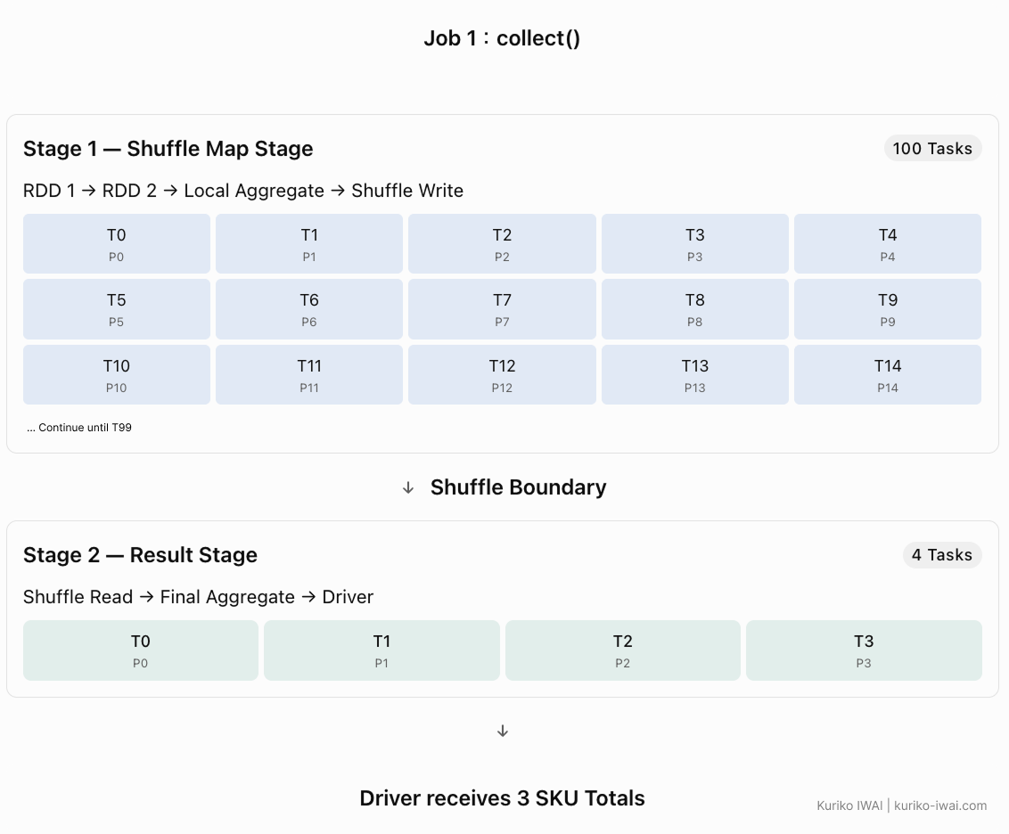
Figure H. Complete RDD lineage graph and dependency flow (Created by Kuriko IWAI)

In Stage 1, each Partition runs computation defined in RDDs 1 and 2 sequentially:

• RDD 1: P0 → RDD 2: P0 → local result P0

• RDD 1: P1 → RDD 2: P1 → local result P1

• …

• RDD 1: P99 → RDD 2: P99 → local result P99

This is called Narrow Transformation where each Partition runs computation independently without exchanging data or computation results with another Partition.

Then, Spark runs Shuffle by SKU because the final aggregation by SKU needs to collect SKU data scattered across all the Partitions.

Lastly, in Stage 2, the 4 Partitions aggregate the results.

Computation which requires Shuffle is called Wide Transformation.

As a result, Step 5 executes 104 Tasks in total:

• Stage 1: 100 Tasks in total.

• Stage 2: 4 Tasks in total.

Note that the total number of Tasks executed in Stage 1 is not 200 (100 Partitions x 2 RDDs) because a Partition handles Narrow Transformation as a single Task.

◼ Step 6. Execute with 14 Task Slots

Our seven 2-core executors provide 14 concurrent one-CPU task slots under the simplified assumptions of 1 CPU allocation per task (Figure C-1).

The table below demonstrates an example of Task allocation to Workers:

Table 4. Worker, Executor, Task, and partition mapping matrix (Created by Kuriko IWAI)

Now, take a look at Task T0 in Stage 1. It follows executions defined in RDD 1 and 2:

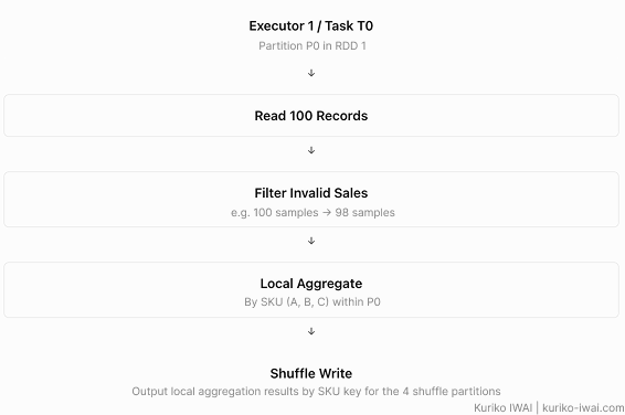
Figure I. Detailed execution mechanics of Task T0 within Stage 1 (Created by Kuriko IWAI)

Other Tasks follow the exact same order in its own Partition.

In our case, Stage 1 has 100 tasks and all slots are available, its execution can be visualized as:

Table 5. Execution scheduling wave breakdown across 14 concurrent task slots (Created by Kuriko IWAI)

Table 5 shows that the system runs 8 waves (100 Tasks / 14 slots).

But note that this is an example of scheduling; it does not indicate that Spark always allocate Tasks in order of the Partition number or in synchronized waves.

Actual scheduling is asynchronous, task durations differ, and locality and resource constraints affect placement. So, if let's say T8 takes longer than the rest in Wave 1, Executor 8 which handles T8 must wait to complete the task, while the rest Executors start to address allocated tasks in Wave 2.

Next, Stage 2 only has 4 Tasks; so the system only uses 4 task slots concurrently, while the rest 10 slots remain unused:

Figure J. Task execution bottleneck during Stage 2 reduce phase (slot underutilization) (Created by Kuriko IWAI)

More executor cores do not automatically make a four-partition stage use 14 CPU cores simultaneously.

◼ Step 7. Returns Computation Results to Driver

Finally, a successful collect() could return the results to the Driver:

1[
2    ("A", 8000),
3    ("B", 10500),
4    ("C", 9200),
5]
6

If Executor fails, Spark can retry failed tasks and, where necessary, recompute missing RDD partitions using lineage.

Recovery behavior depends on the failure and the execution state; a failed task may have new attempts, and stage retries or shuffle-data loss may require additional re-computation.

In a simple example, when Executor 4 in Worker B failed during Task T6 in Stage 1, the Driver assigned another Executor T6.

Execution process using the pyspark framework is quite simple:

1from pyspark.sql import SparkSession
2
3# step 1 - create sparksession
4spark = SparkSession.builder.appName("app1").getOrCreate()
5sc = spark.sparkContext
6
7
8# steps 2 - 4: lazy evaluation
9# step 2 - define rdd 1
10raw_rdd = sc.parallelize(records, 100)
11
12# step 3 - define rdd 2
13filtered_rdd = raw_rdd.filter(lambda row: row[1] > 0)
14
15# step 4 - define rdd 3
16result_rdd = filtered_rdd.reduceByKey(
17    lambda a, b: a + b,
18    numPartitions=4
19)
20
21
22# step 5 to 7 - action (computation)
23result = result_rdd.collect()
24

◼ The JVM Behind PySpark

Apache Spark is primarily built on the Java Virtual Machine (JVM).

As Figure A shows, even when we write Spark applications in Python using PySpark, much of Spark's coordination, scheduling, and distributed execution takes place through JVM-based components.

▫ Driver and Executor JVMs

In a PySpark application, the Python driver communicates with the Spark driver running in the JVM.

The driver coordinates job execution, creates stages, and schedules tasks across executors.

Each Spark executor is typically a JVM process running on a worker node. It manages resources and executes tasks assigned by the driver.

When a task needs to execute Python code, Spark can launch or reuse Python worker processes associated with the executor.

This gives us three important components:

• Python driver: Where application-level PySpark code is written and executed.

• Driver JVM: Coordinates Spark execution and scheduling.

• Executor JVM: Runs Spark tasks and manages execution resources. Python worker processes are involved when tasks require Python execution.

▫ Why the JVM Matters for PySpark Performance

Consider two operations from our sales aggregation example.

RDD transformation:

1filtered_rdd = raw_rdd.filter(lambda row: row[1] > 0)
2

This transformation uses a Python function. During execution, Spark must process the Python function through Python worker processes.

DataFrame transformation:

1filtered_df = sales_df.filter(F.col("qty") > 0)
2

Here, the expression is represented using Spark's structured DataFrame API. Spark can analyze and optimize the expression through its query planning system, rather than executing a Python lambda on every row.

This difference helps explain why built-in DataFrame operations are often more efficient than equivalent Python RDD transformations.

However, DataFrames are not automatically faster in every workload. Performance depends on the operations, data layout, execution engine, serialization overhead, and physical plan.

▫ JVM Heap vs Python Worker Memory

Executor memory configuration also becomes easier to understand once we distinguish JVM and Python processes.

The executor's configured heap memory is used by the JVM for execution and storage-related activities, but it does not represent the complete memory consumption of the executor container.

Additional memory may be required for:

• Python worker processes

• Native memory

• JVM overhead

• Off-heap allocations

• Other execution-related processes

Therefore, as we saw in the previous section, an executor configured with a 3 GiB JVM heap can consume more than 3 GiB of total container memory.

This distinction matters when diagnosing Out-of-Memory (OOM) errors: a JVM heap OOM, a Python worker memory failure, and a container being killed for exceeding its memory limit are different failure modes (Later I'll explain in detail).

A narrow dependency means an output partition depends on a small, bounded number of input partitions, allowing pipelined processing without global redistribution.

A wide dependency means downstream partitions may require data from many upstream partitions, involving an operation called shuffle.

◼ Common Narrow Operations

Table 6-1. Behavioral comparison of common narrow operations in Spark (Created by Kuriko IWAI)

◼ Common Wide Operations

Table 6-2. Behavioral comparison of common wide operations in Spark triggering network shuffle (Created by Kuriko IWAI)

Not every wide transformation always performs a new network shuffle. Dependency types, partitioners, optimizer decisions, existing partitioning, and execution engine behavior matter.

◼ Broadcast Join: Important Exception

Suppose an apparel business joins:

• sales: 500 million rows;

• products: 5,000 product-master rows.

If the product table is small enough, a broadcast join may be appropriate:

1from pyspark.sql.functions import broadcast
2
3joined = sales.join(
4    broadcast(products),
5    on="sku_id",
6    how="left",
7)
8

Rather than shuffle both sides by sku_id, Spark may distribute the small table to executors and join against large-table partitions locally.

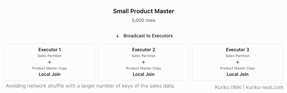
Figure K. Broadcast Join with small product master data (Created by Kuriko IWAI)

Broadcast is not free: distributing and holding the broadcast dataset consumes memory and network bandwidth. Its feasibility depends on actual dataset size and execution plan, not just row counts.

Network shuffle tends to be expensive especially over big data; but the cost of shuffle actually depends on various factors like:

• Data volume,

• Key cardinality,

• Key distribution,

• Serialization,

• Memory,

• Network,

• Disk activity, and

• Aggregation strategy.

◼ Low Cardinality and Map-Side Combine in the Use Case

Our use case only has three SKU keys: A, B, C.

reduceByKey performs map-side aggregation before shuffling data.

Since there are only three distinct SKUs, each input partition produces at most three partial aggregate records:

1Filtered records:                 9,800 records
2Input partitions:                   100
3Possible SKU keys per partition:      3
4Partial key-value aggregates:   up to 300
5

In the partition P0, for example, input is 100 K-V pairs:

("A", 2), ("A", 2), ("B", 3), ("C", 4), ("A", 2), ...

Then output is map-side combine with max. 3 Key-Value pairs:

("A", 50)

("B", 20)

("C", 30)

This would create a maximum 300 K-V pairs (max 3 K-V pairs x 100 input partitions).

This shuffle operation itself is likely not to trigger an OOM error.

▫ How to Investigate If Shuffle Happens

For DataFrame operations, you can check its physical plan to detect shuffle in the plan:

1daily_demand.explain("formatted")
2

Inspect the physical plan for Exchange, aggregation operators, joins, scans, and sorts. Then examine the Spark UI:

• Jobs: What actions/jobs were created?

• Stages: Where are stage boundaries, task counts, and shuffle read/write?

• Tasks: Are there long tails, skewed partitions, retries, or spills?

• SQL / DataFrame execution: What optimized physical operators actually ran?

◼ What Consumes Memory?

Memory consumption spikes in several phases, each of which can trigger OOM errors.

Table 7. Key memory consumers and dominant OOM failure modes in Spark Tasks (Created by Kuriko IWAI)

◼ What Triggers OOM Errors

An OOM error becomes more likely with excessively large per-task state, large partitions, severe skew, insufficient memory, or high simultaneous demand.

Major OOM causes include:

• High cardinality: e.g., millions of SKUs.

• Data skew: Specific key has more data than the rest.

• Large aggregation state: Stores large lists or complex objects by key.

• Lack of sufficient Executor memory.

• Too many parallel Task execution: Many Tasks attempt to consume Executor's memory at the same time.

For example, data skew occurs when some keys or partitions contain far more data or work than others.

A naive aggregation with millions of distinct keys or complex state can generate memory pressure. Even when final output has few records, intermediate processing can still be expensive.

In this particular example, Spark may spill some intermediate data to local disk, reducing memory pressure at a cost in disk I/O and latency. Not all allocations can be spilled, so OOM is still possible.

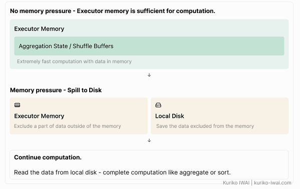
Figure N. Disk spilling behavior during excessive partition memory pressure (Created by Kuriko IWAI)

◼ Diagnosing OOM Errors & Disk Splitting

To avoid OOM errors, we need to check the memory usage:

1. Identify the slow Job and Stage in Spark UI.

2. Inspect Task duration, spill, shuffle metrics, and skew.

3. Inspect the DataFrame physical plan (explain("formatted")) if using DataFrames.

4. Check whether a shuffle, join, unnecessary sort, or repartition drives the cost.

5. Compare changes using actual metrics, not just theoretical task-slot counts.

▫ Partitioning and Parallelism

Too few partitions can leave CPU cores unused and create large tasks. Too many small partitions can incur scheduler overhead and unnecessary shuffle or I/O. The appropriate count depends on dataset size, partition skew, operations, and cluster capacity.

In our example, 100 input partitions can keep 14 slots busy across several task waves. But Stage 2 has only four partitions and therefore underutilizes available slots. Whether increasing reduce partitions helps depends on actual data volume and overhead. For only three SKU keys, four output partitions are already more than enough for the teaching scenario.

▫ Cache and Persist

RDD/DataFrame caching can help when an expensive intermediate dataset is reused across multiple actions. It can also waste memory or cause spilling if data is not reused. Do not cache everything by default. Cache materialization is generally lazy: defining a cache does not guarantee it is populated until an appropriate computation happens.

▫ Data Skew

Look for tasks much slower than their peers, unusually large shuffle reads, excessive spill, and a long tail in stage completion.

Solutions depend on the type of skew: more partitions, alternative join strategies, salting, filtering early, aggregation changes, or adaptive techniques may help in appropriate cases.

The original RDD example helps understand lineage, partitions, and shuffle.

In typical structured ETL, however, the DataFrame API is the preferred starting point because it provides columns, schema information, SQL-like expressions, and optimizer-visible operations.

Below diagram illustrates the relationship:

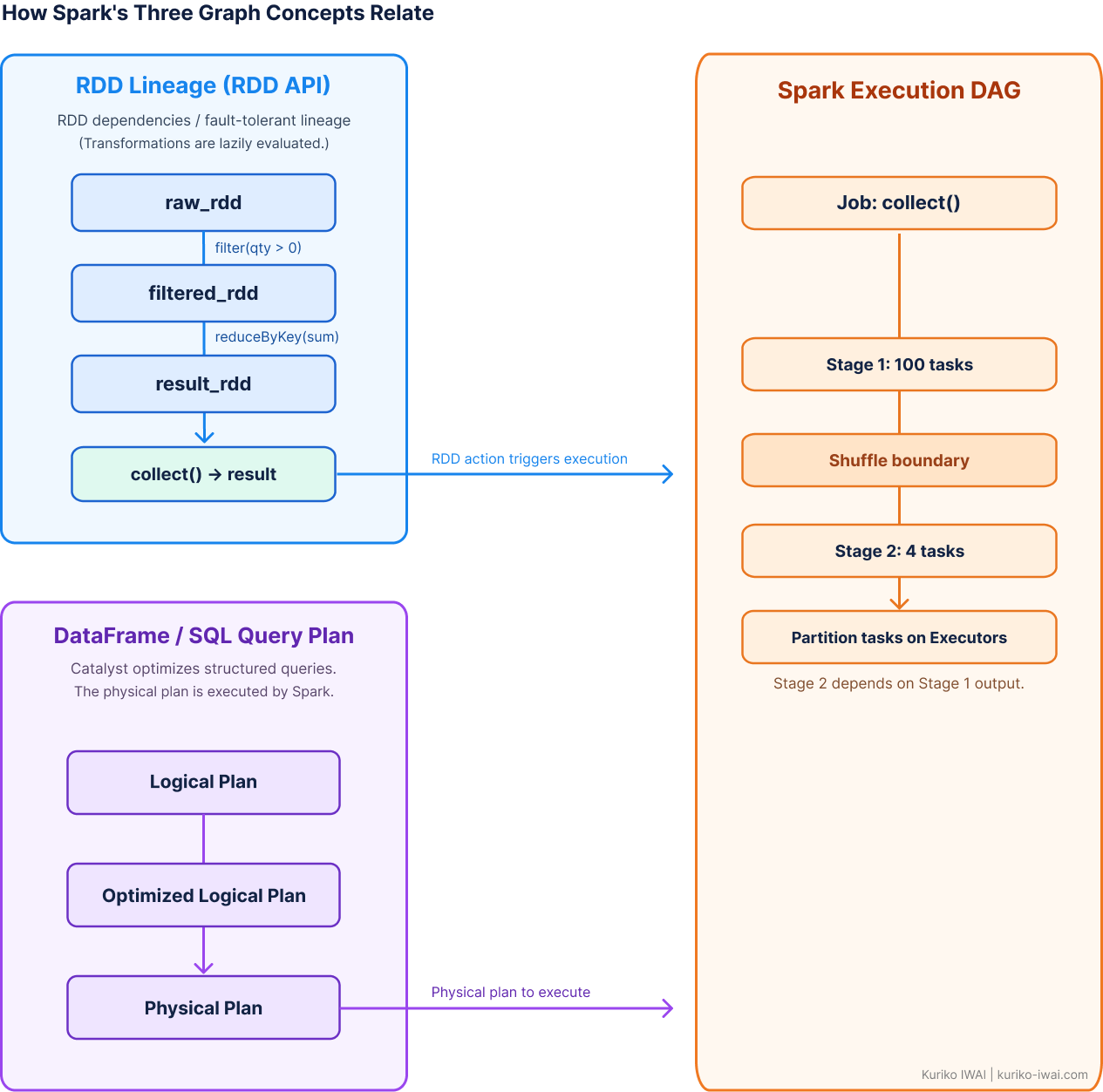
Figure O. How Spark's Graph concepts relate; RDD linage, DataFrame, and Spark Execution DAG (Created by Kuriko IWAI)

This does not mean RDDs can only perform row-wise operations. The core difference is the level of abstraction and how much optimization information Spark receives.

◼ Comparing Actions: RDD vs DataFrame

Let us compare RDD API and DataFrame API, taking the SKU aggregation for an example.

▫ RDD API

The elements are (sku, qty) pairs. Our Python aggregation logic is explicit, and Spark follows RDD dependencies:

1result_rdd = (
2    raw_rdd
3    .filter(lambda row: row[1] > 0)
4    .reduceByKey(lambda a, b: a + b, numPartitions=4)
5)
6
7rdd_results = result_rdd.collect()
8
9# Example:
10# [('A', 8000), ('B', 10500), ('C', 9200)]
11

▫ DataFrame API

Assume sales_df has columns sku (string) and qty (numeric):

1from pyspark.sql import functions as F
2
3result_df = (
4    sales_df
5    .filter(F.col("qty") > 0)
6    .groupBy("sku")
7    .agg(F.sum("qty").alias("total_qty"))
8)
9
10df_results = result_df.collect()
11
12# Example:
13# [Row(sku='A', total_qty=8000),
14#  Row(sku='B', total_qty=10500),
15#  Row(sku='C', total_qty=9200)]
16

Here, both examples solve the same business problem: filtering invalid sales records and aggregating valid quantities by SKU.

And in both cases, collect() triggers Spark execution and returns all resulting records to the Driver.

The difference is in the result representation:

• RDD API: Returns Python elements, such as (sku, total_qty) tuples.

• DataFrame API: Returns structured Row objects with named fields, such as sku and total_qty.

For our example, collecting the results is reasonable because there are only three SKU groups.

However, collect() should be used carefully with large datasets because all returned records must fit in the Driver's memory.

If we only want to inspect a few rows without collecting the complete dataset, the DataFrame API provides show():

1result_df.show(10, truncate=False)
2

This displays up to ten rows rather than returning the entire DataFrame to the application.

Neither collect() nor show() should be confused with a transformation: both are actions that trigger computation.

Here's an overall comparison of RDD and DataFrame APIs:

Table 8. RDD API vs. DataFrame API - feature & abstraction comparison:(Created by Kuriko IWAI)

◼ DataFrame Query Plan

A DataFrame query plan is the sequence of logical and physical steps an execution engine generates to translate operations like filtering or joining into an optimized, executable strategy for retrieving data.

A DataFrame query moves through several representations:

1. Logical plan: A description of the requested operations (scan, filter, group, aggregate).

2. Analyzed and optimized logical plan: Spark resolves references and applies applicable logical optimizations, such as column pruning or predicate pushdown.

3. Physical plan: Spark chooses executable operators, e.g. scans, partial/final aggregates, exchanges, joins, and sorts.

4. Execution: The physical plan is run using Spark's execution mechanisms, ultimately involving tasks on executors.

For the SKU example, the physical plan might include partial hash aggregation → exchange by SKU → final hash aggregation, but actual operators and their order must be checked with explain().

Just like RDD has RDD lineage which defines dependencies between RDD transformations, DataFrame query plan represents a structured query, giving Spark scope for optimization:

1RDD API                           DataFrame / SQL API
2   |                                       |
3   v                                       v
4RDD lineage                 Logical/optimized/physical plan
5   |                                       |
6   +------------------+--------------------+
7                      |
8                      v
9           Spark runtime / scheduler
10            Jobs → Stages → Tasks
11                      |
12                      v
13           Executors process partitions
14

RDDs are not “inside” stages as containers, and stages are not executing inside an RDD object.

Spark constructs execution work from dependencies and physical operators. DataFrame execution may use RDD-based mechanisms internally, but that does not mean users need to manually build RDD lineage when writing DataFrame code.

Local mode: The same concepts can apply when Spark runs on one machine. You simply have fewer physical resources. If the dataset is small, another tool may be more practical, but Spark RDDs remain valid.

The decision to use Spark rather than a single node (Figure A) depends on workload size, infrastructure, and operational needs.

Spark overhead is sum of the following components:

Spark is suitable when the overhead T_{spark} is less than total duration the distributed execution can save.

In other words, even when we deal with 100GB data, a simple computation like our use case (aggregation by 3 SKU only) can be handled by a single node.

Instead, joining big data, multiple window functions, and repetitive feature engineering in machine learning can enjoy the benefits of Spark.

In a case where the existing Spark Cluster is already working, Spark can be suitable because we can save startup overhead.

◼ Data Size Threshold to Use Spark

Data size is one of the significant elements to consider using Spark rather than a single node.

Although there is no universal data-size threshold, as a practical starting point, workloads below 10 GB are worth trying on a single-node engine first.

At tens of gigabytes, benchmark both approaches.

At hundreds of gigabytes or more, distributed Spark becomes increasingly attractive, especially when processing involves expensive joins, aggregations, repeated transformations, or multiple large datasets.

Table 9. Data size threshold ideas for Spark vs single node (Created by Kuriko IWAI)

The goal of Spark tuning is not to maximize partition count or CPU usage independently.

It is to reduce end-to-end execution cost and latency without introducing instability.

In this article, we learn the core relationships in its system:

• Resources: Workers host executors; executors run tasks; configured CPU and memory limit concurrency.

• RDD programming: Transformations produce immutable RDD definitions and lineage; actions trigger computation.

• DataFrame programming: Transformations produce logical query operations; optimization chooses executable physical operators; actions trigger computation.

• Execution: Spark organizes work into jobs, stages, and tasks, and tasks process partitions on executors. Shuffles and other dependencies create coordination boundaries among stages.

• Performance: Partition sizes, skew, shuffle I/O, aggregation state, memory, and task concurrency jointly determine performance. Inspect actual plans and UI metrics before tuning.

Understanding how Spark executes distributed workloads is only the foundation.

In the next article, I'll explore how these concepts apply to building time-series machine learning pipelines on Databricks—and the lessons I wish I'd known earlier.

◼ Appendix - Apache Spark Glossary

Table 10. Apache Spark glossary (Created by Kuriko IWAI)

Written by Kuriko Iwai · Kernel Labs. All images, unless otherwise noted, are by the author. All experimentations on this blog utilize synthetic or licensed data.

FAQ